The compact emitting region in (a) indicates that excitation itself is strongly localized. In (b), the illuminated path generates out-of-focus fluorescence as well as fluorescence near the focus. A confocal detection pinhole can reject much of that unwanted emission from the recorded image; it does not prevent the dye solution from emitting it.
In ordinary one-photon excitation, the local fluorescence-generation rate is approximately proportional to excitation light intensity . In unsaturated two-photon excitation microscopy, it is proportional to . Simultaneous absorption is appreciable only in the high-intensity focal region, generally produced using a pulsed laser. Two lower-energy photons jointly excite the fluorophore; the excitation wavelength is therefore typically substantially longer than in its one-photon experiment. This reduces out-of-focus excitation and permits detection without a confocal pinhole.[ref]
Two-photon laser scanning fluorescence microscopy by Winfried Denk and others. pp. 73–75, quadratic excitation, optical sectioning and pulsed illumination
For a small detection pinhole, the effective confocal point spread function is approximatelyHere each factor denotes an intensity response. Excitation and detection jointly select the focal region. Enlarging the pinhole increases collected signal but weakens axial rejection and changes the effective point spread function. In two-photon excitation microscopy with broad collection, the spatial response is dominated byThe pinhole product and excitation square are different physical mechanisms even when simplified mathematical profiles resemble one another.[ref]
Confocal microscopy (chapter manuscript) by Brad Amos and others. Confocal formation and conjugate focal selection, Fig. 3; discussion of excitation and detection responses
Compare both lateral and axial widths using the actual wavelengths and objective. For a diffraction-limited system, their characteristic scalings arewhere is numerical aperture and is the medium's refractive index. Numerical prefactors depend on the width criterion and high-aperture optical model. Axial resolution is generally worse than lateral resolution. A small confocal pinhole improves axial sectioning and can narrow the lateral response, at the cost of photon throughput.
As a simple Gaussian function example, has squared profile , so its width is reduced by . However, the two-photon illumination spot itself is broader at its longer excitation wavelength. Two-photon excitation is not automatically higher-resolution than confocal microscopy, and ordinary two-photon sectioning is not intrinsically super-resolution. Compare measured point spread functions, pinhole settings, numerical apertures, scattering and optical aberrations, not just the fact that one profile is squared.
The original model figure below separates focal confinement from wavelength-dependent width. It is an illustrative one-dimensional Gaussian function calculation, not a reproduction or quantitative fit of the supplied photograph.
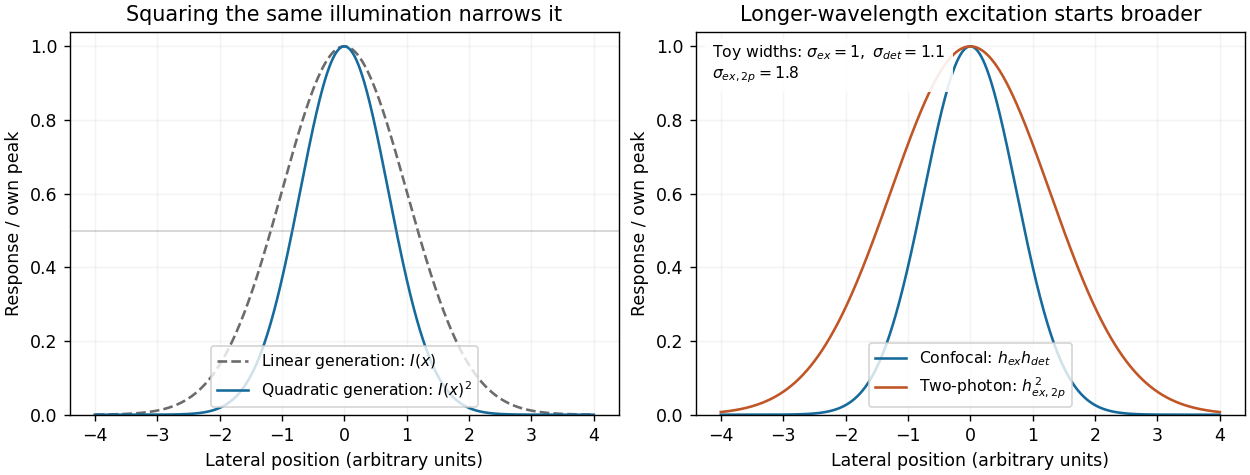
Local excitation nonlinearity and wavelength-dependent point-spread widths
. Left: squaring the same normalized Gaussian illumination narrows the local generation profile. Right: a longer-wavelength illumination profile can remain broader after squaring than an illustrative confocal excitation-times-detection response. All widths are synthetic; peak normalization does not equate photon throughput or excitation dose. Details.
Start with the biological quantity to measure: compartment location, molecular colocalization, fast cell dynamics, deep-tissue activity or nanometre-scale organization. Specify the required field, depth, lateral and axial resolution, temporal sampling and acceptable perturbation before choosing the instrument.
For a thin fixed specimen or a shallow live preparation, confocal microscopy provides flexible multicolour imaging and effective optical sectioning with widely available labels. Adjust the pinhole and dwell time against signal-to-noise ratio, bleaching and speed. Repeatedly scanning a large volume can become too slow, and out-of-focus excitation can damage regions that contribute little useful signal.
For a living scattering specimen, two-photon excitation microscopy often offers better access to depth and confinement of excitation. Longer excitation wavelengths scatter less strongly in many tissues, and broad collection can recover scattered emission without a detection pinhole. These benefits do not eliminate depth-dependent optical aberrations, absorption, heating or focal phototoxicity. Pulsed excitation can also make instrumentation and suitable multicolour excitation more demanding.
If the priority is rapid, gentle volumetric observation of a suitable specimen, consider light-sheet fluorescence microscopy rather than forcing either point-scanning method to cover every use case. If subdiffraction molecular organization is required, consider a suitable super-resolution method and assess its labeling, speed and dose costs.
Finally, calibrate the point spread function in a sample-relevant medium, sample finely enough in all three dimensions, and check registration between colour channels. Match photon collection and exposure to the question, with controls for label-induced changes and photobleaching. The best method meets the biological resolution and timing requirements with sufficient signal and acceptable perturbation; the smallest nominal resolution number alone does not decide.
Stimulated emission depletion microscopy narrows the region allowed to emit detectable fluorescence. A focused excitation pulse or beam populates the excited state. A red-shifted depletion beam with a central intensity minimum drives stimulated emission from the surrounding excited fluorophores. The stimulated photons are rejected from the fluorescence detection channel, leaving spontaneous emission concentrated near the depletion zero. Scanning this small effective emission region builds the image.[ref]
Breaking the diffraction resolution limit by stimulated emission: stimulated-emission-depletion fluorescence microscopy by Stefan W. Hell and others. pp. 780–782, depletion of the outer excitation region and proposed beam geometry
Near an ideal zero, take depletion intensity proportional to squared radius. The radius at which it reaches a saturation scale decreases as the depletion amplitude grows. A common approximate resolution law iswhere is the undepleted characteristic width and depends on fluorophore kinetics and illumination timing. It is an idealized scaling, not a universal instrument calibration. For example, a threefold width reduction needs in this model. The illumination beams remain diffraction limited; nonlinear control of the emitting population creates the smaller effective response.
The cost is high depletion intensity, with possible photobleaching, phototoxicity and heating, demanding fluorophore photophysics, precise beam alignment and maintenance of the central zero. Point scanning limits speed and trades off field size, dwell time and photon statistics. Scattering and aberrations can fill the depletion minimum and degrade performance in depth. A simple lateral doughnut mainly improves lateral resolution; improved axial confinement requires an appropriate three-dimensional depletion pattern. Resolution gain is therefore conditional on usable photons, sample integrity and the actual depletion geometry.
Stochastic optical reconstruction microscopy separates emitters in time rather than shrinking every illuminating spot. Switch only a sparse subset of labeled molecules into a fluorescent state, localize their individual point spread functions, switch or bleach them off, and repeat. Combining many fitted positions reconstructs structure finer than the individual diffraction-blurred spots.[ref]
Sub-diffraction-limit imaging by stochastic optical reconstruction microscopy (STORM) by Michael J. Rust and others. pp. 793–795, sparse activation and localization reconstruction
An interesting application is the neuronal axon. STORM revealed approximately – periodic organization of actin, spectrin and associated proteins, supporting a membrane-associated cytoskeletal architecture that ordinary fluorescence images did not resolve clearly.[ref]
Localization precision improves with detected photons, but reconstructed resolution also depends on label density, label size, drift and reliable separation of emitters. Many frames are needed, so motion and slow acquisition can limit live imaging. Multiple localizations of one blinking label must not automatically be counted as multiple molecules. A precise molecular fit and a faithful reconstructed biological structure are related but distinct achievements.
Articles by others on the same topic
There are currently no matching articles.