Write the parameters as , where is the fraction of molecules in component , is its mean current, and is its current standard deviation. The mixture weights satisfy and . Thus six displayed parameters represent five independent degrees of freedom.
Assigning component 1 to modified molecules makes the inferred modification fraction. That biological assignment needs a reference or other identifying information: exchanging both component labels leaves the Gaussian mixture distribution unchanged. In the illustrated multi-sample model, component locations can be shared while the sample-specific fractions differ; this is different from fitting unrelated means to every sample.
The probability density function isEvery term is nonnegative because its weight is nonnegative, its scale is positive and its exponential is positive. By linearity of the integral and normalization of each normal distribution,Thus is nonnegative and integrates to one. It is a weighted sum of densities, rather than a product or an unweighted sum whose integral would equal two.
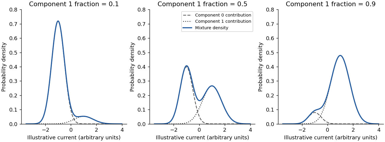
Illustrative Gaussian mixtures with shared component distributions and different modification fractions
. Details. 
A five-base current measurement alone does not guarantee identification of one modified base in every sequence. At GGACT there is only one adenosine in the window, so attributing an established adenosine-specific modification to that A is plausible. That does not establish a universal resolution claim.
For a counterexample, consider a window containing two candidate adenosines. If modifying either position produces indistinguishable current distributions, its signal cannot identify which A changed. Overlapping windows, sequence context, calibrated modification signatures or external evidence may resolve some ambiguities, but they are extra information. This is an identifiability issue: estimating the fraction in a shifted current component is not automatically the same as identifying its molecular cause or exact position.
Add direct sample labels and distinguish line styles or marker shapes, rather than encoding sample identity solely by colour. The sample identities would then remain visible in greyscale and for readers with colour-vision deficiencies. Larger axis text and a high-contrast palette would also improve readability. An accessible text description should state the comparison and principal result, rather than merely saying that the figure contains coloured curves.
Define the evaluation universe first, including which sufficiently covered loci were eligible for both methods. Relative to the reference assay's labels,The true positive rate is the fraction of reference-positive loci retained by xPore; the false positive rate is the fraction of reference-negative loci incorrectly retained. The latter is not the fraction of xPore calls that fail validation.
An imperfect reference assay can miss real modifications. “False positive” here therefore means disagreement with that reference, not independently demonstrated absence of a modification. Restricting the universe differently for the two denominators would invalidate the comparison.
Choose a cutoff on the ranked score and call every eligible locus above it positive. Compare those calls with the fixed reference labels, count , and plot . Repeating over cutoffs generates the receiver operating characteristic.
A very restrictive cutoff starts near ; a cutoff calling everything positive ends at . The reference labels and eligible locus set must stay fixed during this sweep. Tied scores need a consistent treatment. A single cutoff gives one operating point, whereas the curve describes the trade-off across many possible cutoffs.
A good receiver operating characteristic rises toward the upper-left corner: many reference-positive loci are detected while few reference-negative loci are accepted. The area under the ROC curve summarizes this discrimination over cutoffs. Higher is better in the stated score direction; perfect separation gives one. The displayed value near 0.86 indicates substantial ranking discrimination against this reference.
The area can also be interpreted as the probability that a randomly chosen positive receives a higher score than a randomly chosen negative, with half credit for ties. It does not select a cutoff or demonstrate that most retained calls are correct: those practical questions also depend on prevalence and the relative costs of errors.
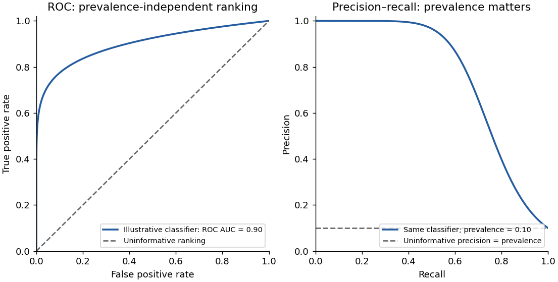
The same illustrative classifier viewed through ROC and precision–recall curves at ten percent prevalence
. Details. 
The diagonal means no ranking discrimination against the reference labels, with ROC area 0.5. At every operating point on that diagonal, the fraction of positives accepted equals the fraction of negatives accepted. A score independent of the true label has this expected behaviour.
This does not imply that exactly half of all individual predictions are correct: an imbalanced dataset can have high accuracy by always predicting the majority class. It also does not establish biological absence of signal; it describes what the evaluated score extracts relative to the chosen reference and dataset.
The two quantities areClassification precision asks how many retained calls agree with the positive reference; classification recall asks how much of the positive reference set has been recovered. Recall is the true positive rate. Increasing recall by accepting more loci can reduce precision through additional false positives.
If positive prevalence is , thenThus prevalence matters: good ROC discrimination need not give high precision when true positives are rare. A precision–recall area must be judged against its own prevalence-dependent baseline; it is not numerically interchangeable with ROC area.
It is a useful depletion control, but not an automatically modification-free negative control. A nominal knockout may retain functional products, and loss of one writer does not establish absence of every relevant RNA modification. Calling the sample completely negative requires independent validation of the molecular state being used as ground truth.
This distinction has direct experimental support: alternatively spliced functional METTL3 products have been found in some nominal knockout lines.[ref]
Alternative splicing of METTL3 explains apparently METTL3-independent m6A modifications in mRNA by Hui Xian Poh and others. Abstract and Results: residual functional METTL3 isoforms in purported knockout cells
That result identifies a possible failure mode; it does not prove that this particular sample has the same defect. A modification-free reference preparation and an independent chemical measurement would strengthen the interpretation.Pooling can erase between-replicate variation. One unusually well-covered or highly modified sample can dominate the pooled estimate, hiding an inconsistent biological response. If individual reads are then treated as independent biological replicates, uncertainty can be understated through pseudoreplication.
A better analysis retains replicate identity and models sample-to-sample variation, while allowing information to be shared about suitable common component parameters. Pooled performance on a larger dataset can be useful, but should not substitute for evidence that the result reproduces across independent biological samples.
Use small multiples with consistent axes, direct cutoff labels and distinguishable line styles, with an inset enlarging the low-false-positive-rate region of the ROC curves. Add a compact summary of area versus minimum read count with uncertainty intervals and the number of eligible loci retained at each cutoff. This would make the modest ROC-area change and larger precision–recall-area change easier to assess than several nearly overlapping colours.
A coverage restriction also changes which loci are evaluated. For a clean comparison, show performance on a common locus subset as well as the practical retained set; otherwise an apparent improvement may partly reflect exclusion of difficult loci or a changed positive prevalence.
The panel supports feasibility in these samples, but not the full strength or generality of the claim. The method produces modification estimates for three patient samples, and the displayed selected genes generally have higher estimates than the knockout controls. That is evidence that an analysis can be performed and yields biological-looking contrasts.
The comparison simultaneously changes cell background, disease status and potentially sequencing conditions. The displayed genes were selected for high estimated modification, creating selection bias; the same estimates do not independently validate their accuracy. The panel also does not itself show input-RNA amounts, uncertainty, or performance across controlled input levels. It therefore cannot alone establish reliable low-input performance across genetically diverse clinical samples or disease-specific modification differences.
Two useful changes would be:
- Show patient estimates together with matched, relevant cell-type controls and an independent measurement of modification at prespecified or held-out loci. Display uncertainty and all evaluated loci, or state a selection rule independent of the reported contrast. This separates genuine agreement from selection of high xPore values and from unrelated cell-background effects.
- Add performance across measured RNA-input levels for the same biological materials, with biological and technical replication, read coverage and failure rates reported. This tests the low-input part of the claim directly rather than inferring it from the heatmap.
A single additional knockout row would not address both independent accuracy and input dependence.
Articles by others on the same topic
There are currently no matching articles.