Past exam of the theoretical physics I course of the University of Cambridge / 2016 / Paper 1 / 3

Treat $\varphi$ and ${\varphi }^{\ast }$ as independent variables during variation. With Minkowski metric $(+---)$, differentiation with respect to ${\varphi }^{\ast }$ givesThe Euler-Lagrange field equation is therefore $\square \varphi +2ie{A}^{\mu }{\partial }_{\mu }\varphi +ie({\partial }_{\mu }{A}^{\mu })\varphi +m^2\varphi =f$. The static purely temporal potential has ${\partial }_{\mu }{A}^{\mu }={\partial }_{t}V=0$, givingvariation with respect to $\varphi$ gives $(\square -2ie{A}^{\mu }{\partial }_{\mu }+m^2){\varphi }^{\ast }=f(t)$. This is the complex conjugate equation when the driving force is real, as is required for the supplied lagrangian density to be real. For a complex driving amplitude a real source term would instead require conjugate coefficients. The interaction supplied here is linear in the external potential: adding the $e^2{A}_{\mu }{A}^{\mu }|\varphi {|}^2$ term from full minimal coupling would change the problem and its equation of motion.

Time independence of $V$ makes the Green function depend on $t,t^{\prime }$ through $\tau =t-t^{\prime }$. A spatially varying potential does not imply spatial translation invariance. Fix ${\mathbf{r}}^{\prime }$ and set $\mathbf{x}=\mathbf{r}-{\mathbf{r}}^{\prime }$; write the Fourier coefficient more fully as $G_{{\mathbf{r}}^{\prime }}(\mathbf{k};\omega )$. The source position is an implicit parameter in the printed notation. DefineThe ordinary derivative terms transform into $(-{\omega }^2+k^2+m^2)G_{{\mathbf{r}}^{\prime }}$. The product $V{\partial }_{t}G$ becomes a convolution, and $2ie(-i\omega )=2e\omega$. More explicitly, insert both inverse spatial Fourier transforms into $VG$: the integral over $\mathbf{x}$ enforces $\mathbf{q}+{\mathbf{k}}^{\prime }=\mathbf{k}$. The transformed delta source is one, leavingThis is a source-position-dependent Fourier Green function. Dropping the explicit ${\mathbf{r}}^{\prime }$ subscripts recovers the requested notation with exactly the potential transform defined in the source. No assumption of a homogeneous potential is needed. The factor $(2\pi {)}^{-3}$ and the source-position phase are necessary for the stated Fourier convention.

The delta function in the specified convolution kernel collapses the ${\mathbf{k}}^{\prime }$ integral to $-i\gamma G$. Set $\lambda =e\gamma$ and ${\omega }_0^2=k^2+m^2$. ThenThere is a change of assumptions here: the specified kernel is the transform of $V=-i\gamma$, which is not real. These later parts define a formal analytic continuation to an effective damped equation, $[{\partial }_{\tau }^2+2\lambda {\partial }_{\tau }+{\omega }_0^2]G=\delta (\tau )$; they cannot simultaneously describe the earlier real external potential. The following pole analysis uses that continued operator.

Completing the square gives $D(\omega )=-(\omega +i\lambda {)}^2+({\omega }_0^2-{\lambda }^2)$, soFor $e>0$, hence $\lambda >0$, the underdamped regime has two poles at $\pm \Omega -i\lambda$, with $\Omega =\sqrt{k^2+m^2-{\lambda }^2}>0$. Both lie below the real axis. In the overdamped regime they lie on the imaginary axis at $-i(\lambda \mp \kappa )$, where $\kappa =\sqrt{{\lambda }^2-k^2-m^2}<\lambda$ for $k^2+m^2>0$; both are again below the real axis. At equality they coalesce into a double pole at $-i\lambda$. If $m<|\lambda |$, the crossover occurs at $k_c=\sqrt{{\lambda }^2-m^2}$; increasing $k$ moves the two imaginary poles together and then apart horizontally. If $m>|\lambda |$, every $k$ is underdamped; if equal, only $k=0$ is critical.

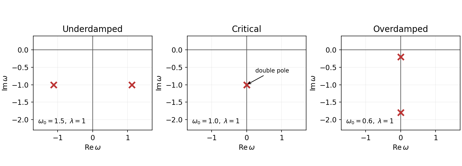
The sign of $e$ is not specified: for $e<0$ all nonzero-frequency poles are instead in the upper half-plane, describing antidamping; for $e=0$ they lie on the real axis and a causal prescription is required. When $m=k=0$, one pole is at zero even for nonzero $\lambda$ and a real-axis prescription is again needed. The figure uses illustrative $\lambda =1$, not supplied numerical data.

Let $\tau =t-t^{\prime }$ and $\Omega =\sqrt{k^2+m^2-{\lambda }^2}>0$. First take $\lambda =e\gamma >0$. Since $|e^{-i\omega \tau }|=e^{\tau \mathrm{Im}\omega }$, close the contour below for $\tau >0$, and above for $\tau <0$. On the chosen semicircle the exponential is bounded and the denominator grows as $R^2$, so the arc integral tends to zero. The upper contour encloses no pole, giving $G=0$ for $t<t^{\prime }$. The lower contour is clockwise, hence the real-axis integral divided by $2\pi$ is $-i$ times the sum of residues. Since $D^{\prime }({\omega }_{+})=-2\Omega$ and $D^{\prime }({\omega }_{-})=2\Omega$, that sum isThusThis is the causal Green function of a damped oscillator. Its value is continuous through $\tau =0$, and its derivative jumps from zero to one; integrating the differential equation through zero verifies the delta-source normalization and the residue sign. The limits are $H(\tau )\tau e^{-\lambda \tau }$ at critical damping and $H(\tau )e^{-\lambda \tau }\sinh (\kappa \tau )/\kappa$ in the overdamped regime.

For completeness, if the unspecified charge has $e<0$, the same real-axis integral instead encloses upper poles for $\tau <0$ and gives $-H(-\tau )e^{-\lambda \tau }\sin (\Omega \tau )/\Omega$, an advanced Green function. A causal growing response would require an inverse-Laplace contour above those poles, not the stated real-axis Fourier integral. At $e=0$ the real-axis integral needs a pole prescription; shifting both poles below it gives the retarded zero-damping limit. These distinctions are necessary because $\gamma >0$ alone does not fix the sign of damping.