Original source: Cambridge FOI 2023/399 released PDF, physical pages 417–420.
Write the bead position in Cartesian coordinates as . Differentiation gives , while the free particle has . Thus the kinetic energy is the sum of these squared speeds weighted by half the respective mass. The squared spring length isA spring obeying Hooke's law with zero natural length has potential energy . Consequently , and deleting the additive constant givesThe spring length is the straight separation of its endpoints, not distance measured along the helix. The fixed frictionless constraint is already incorporated by using the generalized coordinate ; it supplies no extra potential energy.
Set and . Applying the Euler-Lagrange equations separately to givesFor example, whereas ; these signs also follow from equal and opposite spring forces projected on the permitted bead motion. The angular particle equation can equivalently be written . The factor is the bead's inertia with respect to the helical coordinate, rather than its moment of inertia about the axis alone.
The continuous transformation , , , moves both endpoints by the same screw motion and preserves the fixed helix. Both and are unchanged, so . Noether theorem therefore givesThis is the Noether conserved quantity for a mechanical point symmetry applied to helical symmetry. In physical Cartesian terms it equals total angular momentum plus times total linear momentum: the bead contributes . Neither pure axial translation nor pure axial rotation preserves the fixed coil separately. Their conserved combination is a consequence of the helical symmetry, not two independently conserved momenta. Substitution of the four equations of motion verifies .[ref]
In the negligible bead-mass limit the bead contribution to vanishes. Since the particle starts at rest, , and hence . Assume and a regular massless limit. Integrating along the trajectory giveswhere is the closed projection onto the plane perpendicular to the coil axis. The given final and ensure that this projection closes. Green's theorem identifiesThus is the signed area enclosed by the transverse projection, positive for counterclockwise traversal viewed from positive . Self-intersecting projections contribute their winding-weighted areas; it is neither an unsigned area nor an area of a surface in three dimensions. For , a positive signed area gives negative axial displacement. This is signed-area displacement under a helical constraint: returning to the same projected coordinates can leave a nonzero axial displacement.
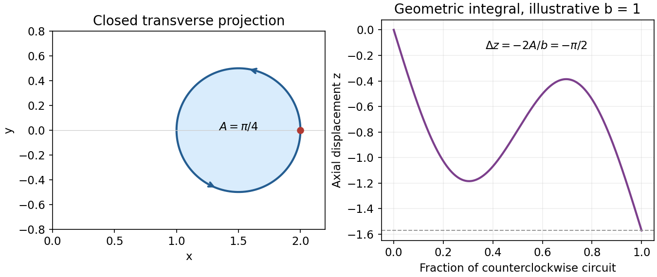
Signed transverse area and the associated axial displacement for an illustrative closed projection
. Details. The plotted loop illustrates the geometric integral only; it is not asserted to be a particular spring trajectory.
Use natural units and the Minkowski metric , with and . Then , , and . The electromagnetic field tensor is an antisymmetric tensor, which gives givesintegration by parts in the action, with the variation vanishing on its boundary, yields . Independent variations of the four components therefore give . The time component is ; the spatial components are . These are the two source-free Maxwell equations obtained dynamically. The other two, and , follow identically from , through the Electromagnetic Bianchi identity. They are not additional Euler-Lagrange field equations.[ref]
In the same Minkowski metric and electromagnetic units, . Differentiating givesTo simplify the last two terms, contract with . Its first and third terms are equal, and its middle term is . Raising therefore gives . The cancellation leavesThis is the electromagnetic stress-energy divergence identity in rationalized units. As a sign check, is positive and is the Poynting vector. The integrated four-momentum is conserved if the boundary flux vanishes. With matter sources, the electromagnetic field alone instead obeys : energy and momentum transfer to matter restore conservation of the total stress-energy tensor.
Hold fixed while varying . With the specified convention , the two matter variations are and . ThusAdding the Maxwell variation from part (a) gives . ConsequentlyExpanding the gauge covariant derivatives supplies a useful convention check:In particular, the last sign is negative for the specified plus sign in . Reversing that convention requires consistently changing the phase transformation and current conventions as well. This current is the matter source in scalar electrodynamics; its dependence must not be dropped.
Take the constant-parameter subgroup of the local transformation: , , . The momenta conjugate to the complex scalar field gradients are and . Noether theorem givesThe scalar field equations are and their complex conjugate. Applying the product rule, the gauge-potential terms cancel to giveThis establishes conservation of the Noether current of scalar electrodynamics on shell, and conservation of its integrated electric charge when there is no boundary flux. An arbitrary function describes gauge redundancy; the associated Noether second theorem supplies an identity among Euler-Lagrange field equations, rather than a distinct physical charge for each function. Indeed its on-shell current can be written . The antisymmetric tensor makes its divergence vanish. Independently, differentiating the Maxwell equation also gives , confirming compatibility with the matter derivation.[ref]
Quantum Field Theory by David Tong. §1.3.4, internal phase symmetry; §6.1, gauge symmetry and its constant subgroup
Treat and as independent variables during variation. With Minkowski metric , differentiation with respect to givesThe Euler-Lagrange field equation is therefore . The static purely temporal potential has , givingvariation with respect to gives . This is the complex conjugate equation when the driving force is real, as is required for the supplied lagrangian density to be real. For a complex driving amplitude a real source term would instead require conjugate coefficients. The interaction supplied here is linear in the external potential: adding the term from full minimal coupling would change the problem and its equation of motion.
Time independence of makes the Green function depend on through . A spatially varying potential does not imply spatial translation invariance. Fix and set ; write the Fourier coefficient more fully as . The source position is an implicit parameter in the printed notation. DefineThe ordinary derivative terms transform into . The product becomes a convolution, and . More explicitly, insert both inverse spatial Fourier transforms into : the integral over enforces . The transformed delta source is one, leavingThis is a source-position-dependent Fourier Green function. Dropping the explicit subscripts recovers the requested notation with exactly the potential transform defined in the source. No assumption of a homogeneous potential is needed. The factor and the source-position phase are necessary for the stated Fourier convention.
The delta function in the specified convolution kernel collapses the integral to . Set and . ThenThere is a change of assumptions here: the specified kernel is the transform of , which is not real. These later parts define a formal analytic continuation to an effective damped equation, ; they cannot simultaneously describe the earlier real external potential. The following pole analysis uses that continued operator.
Completing the square gives , soFor , hence , the underdamped regime has two poles at , with . Both lie below the real axis. In the overdamped regime they lie on the imaginary axis at , where for ; both are again below the real axis. At equality they coalesce into a double pole at . If , the crossover occurs at ; increasing moves the two imaginary poles together and then apart horizontally. If , every is underdamped; if equal, only is critical.
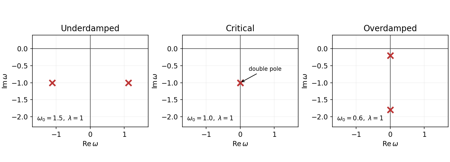
The sign of is not specified: for all nonzero-frequency poles are instead in the upper half-plane, describing antidamping; for they lie on the real axis and a causal prescription is required. When , one pole is at zero even for nonzero and a real-axis prescription is again needed. The figure uses illustrative , not supplied numerical data.
Let and . First take . Since , close the contour below for , and above for . On the chosen semicircle the exponential is bounded and the denominator grows as , so the arc integral tends to zero. The upper contour encloses no pole, giving for . The lower contour is clockwise, hence the real-axis integral divided by is times the sum of residues. Since and , that sum isThusThis is the causal Green function of a damped oscillator. Its value is continuous through , and its derivative jumps from zero to one; integrating the differential equation through zero verifies the delta-source normalization and the residue sign. The limits are at critical damping and in the overdamped regime.
For completeness, if the unspecified charge has , the same real-axis integral instead encloses upper poles for and gives , an advanced Green function. A causal growing response would require an inverse-Laplace contour above those poles, not the stated real-axis Fourier integral. At the real-axis integral needs a pole prescription; shifting both poles below it gives the retarded zero-damping limit. These distinctions are necessary because alone does not fix the sign of damping.
For the isotropic zero-field classical Heisenberg model of a ferromagnet, the analytic vector Landau expansion uses the Cartesian components of the vector order parameter near . rotational symmetry makes its scalar terms functions of . Global spin inversion symmetry also requires . Through fourth order this givesA positive quartic coefficient stabilizes the unconstrained truncated free energy. The disordered phase has and its minimum at ; the aligned phase has and a minimum at nonzero . At the continuous transition . The attractive alignment interaction supplies an energetic tendency toward negative quadratic curvature; orientational entropy favors the disordered phase at high temperature, so the sign of is a free-energy question rather than a consequence of the pair energy alone.
The analyticity assumption matters: the variable printed as is a nonnegative magnitude, so reversing does not send that scalar to . Terms proportional to or would be rotationally invariant but nonanalytic at the vector origin. Standard analytic Landau theory excludes them. Without that assumption, the stated pair symmetry alone would not exclude odd powers of the magnitude.[ref]
Statistical Field Theory by David Tong. §1.2, small-order-parameter expansion; §4.2, rotationally invariant vector free energy
Differentiation gives . For the origin is the global minimum; for , has and . Therefore, close enough to the transition for the quartic expansion to apply,The order parameter approaches zero continuously with mean-field critical exponent : the transition is continuous. In the aligned phase a particular direction is chosen. The vector-spin rotation symmetry is spontaneously broken from to , or from to including reflections. The manifold of vector order parameter directions is a sphere, so this is not just a two-state sign choice.[ref]
Statistical Field Theory by David Tong. §4.2, Heisenberg model and the continuous set of ordered directions
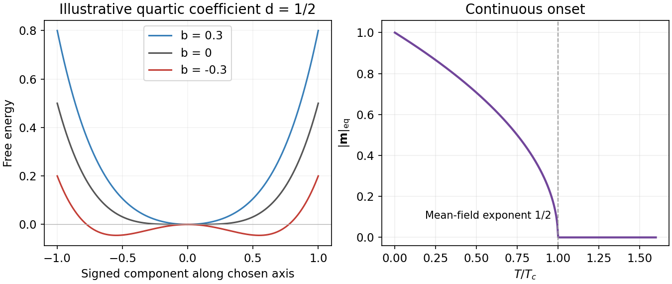
The plot uses illustrative and temperature measured in units of . A unit-spin average must satisfy ; if the quartic model is used literally far below the transition, its constrained minimum is . In practice the near-transition expansion is not a controlled prediction of deep low-temperature saturation. Also, a finite zero-field statistical ensemble that averages all directions has even below ; the curve describes the magnitude in a selected ordered state, obtained by appropriate boundary conditions or the thermodynamic limit before removing a small magnetic field.
The independent head-tail reversal symmetry means that the squared dot product interaction energy is unchanged when any individual is replaced by . All configurations , with independently, attain the aligned ground-state pair energy. There is consequently no energetic preference for either end of a molecular axis. Averaging over these equally weighted signs gives and even in the nematically ordered phase. The surviving order is the unoriented axis, represented by a nematic director with . A second-moment tensor can detect this order while a polar vector cannot.[ref]
Lectures on Landau Theory of Phase Transitions by Peter D. Olmsted. §4.3, printed pp.10–11, head-tail equivalence and the tensor order parameter
The word “always” needs the statistical ensemble or apolar interpretation: it is not an identity for each finite configuration. For example, choosing all is also a ground-state representative and gives . In an unbiased sign statistical ensemble the typical residual polar vector has size of order , because for these independent ground-state signs. This does not make polar order an equilibrium nematic order parameter. The tensor below is unchanged by each sign flip and thus removes the arbitrary labeling of rod ends.
Contract the two Cartesian indices and use the unit length of each molecular orientation:This is exact for each configuration, with no ensemble average assumption. The nematic order parameter is also a real symmetric second-rank tensor. Under a common rotation it transforms as , so its powers give rotational invariants of a symmetric traceless tensor by the cyclic property of the trace. It is unchanged by independent sign flips of the molecular vectors, explaining why it is adapted to nematic rather than polar order.
Choose a basis whose first axis is . The tensor with uniaxial nematic order then has eigenvalues . Hence , and . Substitution givesFor , remains a local minimum with curvature . Its nonzero stationary points satisfy , soThey first appear at as a stationary inflection point; for more negative , is a local maximum and a local minimum. The latter is initially metastable, becomes degenerate with at , and then becomes the global minimum as decreases further. This is a first-order transition in a cubic-quartic Landau potential: the order changes discontinuously. The saddle-node bifurcation creating a local minimum is not the coexistence condition. The isotropic minimum never loses local stability in this fixed positive- scan.
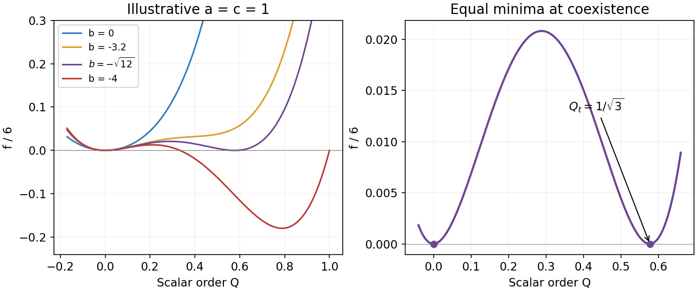


The illustrative plots set and show . A cubic invariant is permitted because head-tail reversal leaves unchanged; it does not implement . The physical range of a uniaxial nematic order parameter imposes ; the usual small-order-parameter Landau result assumes the displayed minimum lies in that interval. The unrestricted quartic graphs express the intended Landau model, with the effect of enforcing the bound stated in part (f).[ref]
Lectures on Landau Theory of Phase Transitions by Peter D. Olmsted. §4.3, printed pp.11–13, tensor invariants and cubic-term-driven coexistence; coefficient normalization here is derived from this paper's definition of
At coexistence a nonzero must be stationary and have the same free energy as . Dividing by and by givesEliminating yields and then . The allowed nonpositive root therefore givesAs is decreased through , the equilibrium scalar order jumps from for to just on the side. At both values coexist; the stable aligned branch below it is from part (e). As a global-minimum check, at coexistenceThere are two equal minima and a barrier at , of height . Comparing these minima, rather than finding only the stationary-point discriminant, determines the transition.
This is the unrestricted Landau answer, compatible with the physical range of a uniaxial nematic order parameter when so that . If one instead enforces for arbitrary positive coefficients, negative cannot win for , and bounded quartic nematic coexistence minimizes over . For its minimum is at the boundary, giving and a jump . No coefficients were supplied to choose this boundary case; the near-transition Landau approximation normally uses the interior result.
Articles by others on the same topic
There are currently no matching articles.