The free complex Proca field has Poincaré symmetry, with transforming as a spacetime four-vector, and the global internal U(1) symmetryThe free theory is also invariant under charge conjugation and the usual parity and time reversal transformations of a vector field. The internal real-field description consists of two equal-mass real Proca fields, with an symmetry containing the phase rotations and charge conjugation.
A gradient shift of leaves unchanged, because partial derivatives commute. It changes the mass term byThis is generally nonzero: for example, and real produce . Thus a massive Proca field has no such gauge symmetry. The massless kinetic term alone would have it.
Treat and as independent variables in the Euler-Lagrange equation. Varying gives the Proca equationThe divergence of its first term vanishes by antisymmetry and commuting partial derivatives. Since , it follows that . Substitution into the original equation givesThe complex-conjugate variation gives , hence and .
For an on-shell plane wave , the Lorenz constraint in Proca theory is . In the rest frame it sets , leaving three complex particle polarizations. Thus the complex Proca field has three independent complex dynamical components, or six real ones; its quantized particle and antiparticle each have three physical particle polarizations. The conjugate field is not another unrelated classical field.
Use the upper-index coordinates specified in the paper. Differentiation of the Lagrangian density gives the canonical momentaIn particular, and . No time derivative of appears, so the zero momenta are primary constraints, not invertible equations for .
For spatial indices, , so , with the conjugate relation for . AlsoThe Legendre transform for the complex Proca Hamiltonian, therefore givesRepeated spatial indices in the positive product denote an ordinary three-component sum. A total Hamiltonian additionally includes multipliers for .
The Hamiltonian printed in the source cannot follow from the given complex Lagrangian density: its missing conjugations, mass coefficients and spatial mass sign are inconsistent. A concrete check is spatially uniform initial data , , with all canonical momenta zero. The correct Hamiltonian density is , while the printed expression gives . These data satisfy the initial constraints and evolve as a spatially uniform massive oscillator. Thus the discrepancy is not a harmless surface term or a different complex-field normalization.
Preserve the primary constraints using the corrected Hamiltonian from solution. After a spatial integration by parts, the terms in its density are . Hamilton's equations giveWith the definitions of in the paper, the actual massive Gauss law is thereforeThis is also the component of the Proca equation. The zero right-hand sides printed in the source apply only to the massless theory or to special configurations with .
For a concrete counterexample, take , , and the longitudinal on-shell plane waveIt satisfies , but and . Imposing the printed zero-divergence condition would incorrectly remove the physical longitudinal particle polarization.
The naive equal-time canonical commutation relations would bewith all coordinate-coordinate, momentum-momentum and mixed conjugate-sector commutators zero before enforcing constraints. But the relation contradicts as an operator identity: its left side would vanish and its right side would not.
The primary zero-momentum constraints and the secondary massive Gauss laws form second-class constraints; their Poisson bracket matrix contains nonzero terms proportional to . They must be eliminated, or treated using a Dirac bracket, before quantization. In a reduced description the three complex spatial coordinates and their momenta are canonical, whileare dependent operators. Substituting them in the integrated Hamiltonian gives the positive density, up to a surface term,Thus the problem is a constrained choice of canonical variables, not an absence of a consistent free quantum field theory.
Introduce the electromagnetic electromagnetic field tensor and the charged vector field strength , with . Minimal coupling givesUnder and ,Consequently the required relation isThen , its complex conjugate transforms oppositely, the mass bilinear is invariant, and . Each term in the total Lagrangian density is therefore invariant under the electromagnetic U(1) gauge symmetry. This phase gauge symmetry does not reinstate the broken gradient-shift gauge symmetry of the massive field itself.
Set , so . Expanding the minimally coupled Lagrangian density givesThus there is a derivative cubic interaction vertex of order , and a quartic interaction vertex of order . There is no pure contact term in this minimal coupling theory, nor an Abelian three-photon interaction vertex.
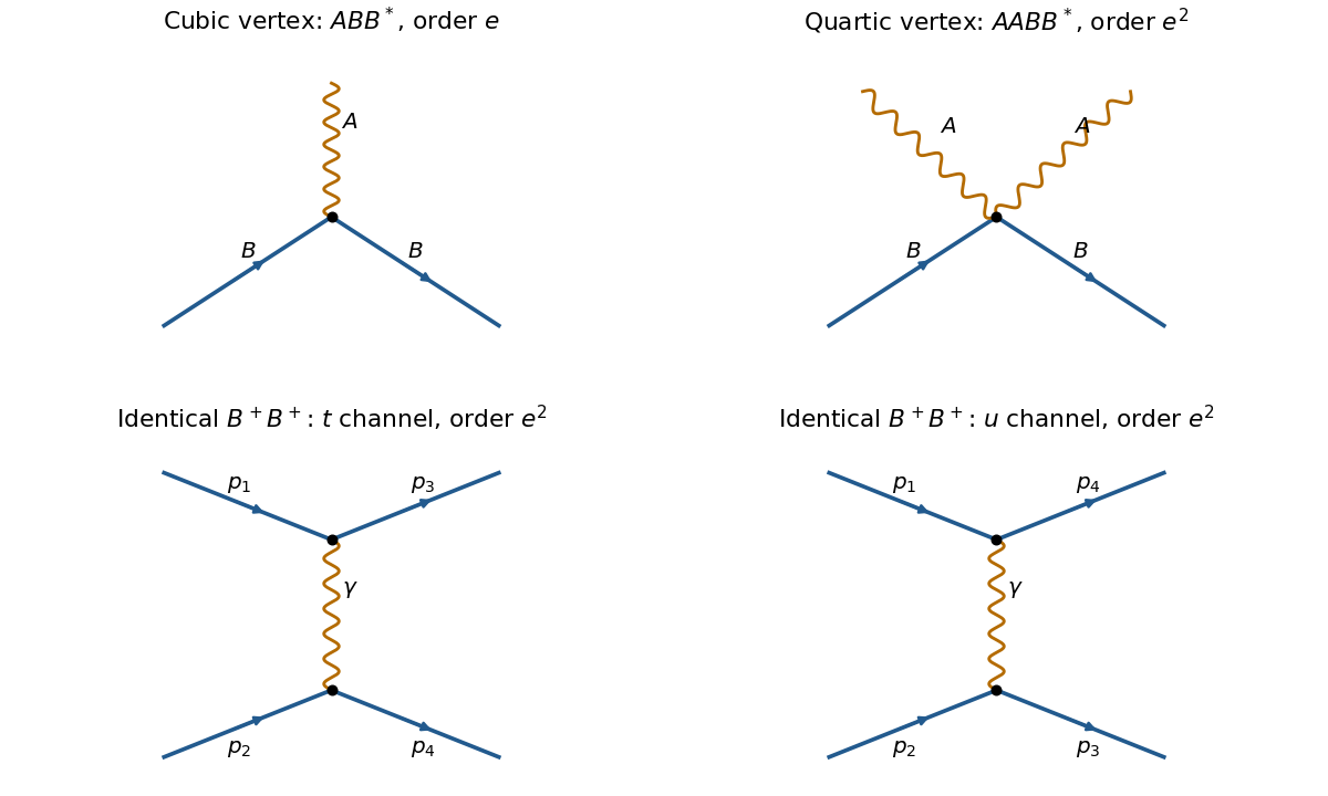
Cubic and quartic charged-vector vertices, and the two photon-exchange channels for identical charged vector bosons
. Details. 
The straight arrowed lines in the original schematic denote charged massive vector bosons; the wavy lines denote photons. For two identical positively charged vector bosons, the leading scattering amplitude has the order- -channel photon-exchange Feynman diagram, together with its -channel interchange required by identical bosons. A quartic interaction vertex cannot directly attach four external massive vector bosons. For a particle-antiparticle incoming pair, the leading channels instead are -channel exchange and -channel photon annihilation. The shown arrows track charge flow; an outgoing charged particle corresponds to the conjugate field at a vertex.
Articles by others on the same topic
There are currently no matching articles.