Functional programming, design and analysis of algorithms (4208)

a

Solution

The two constructors encode a natural number by its number of successors. Structural recursion replaces the zero constructor by zero and every successor by one addition:

convert :: Natural -> Integer
convert Zero     = 0
convert (Succ n) = 1 + convert n

Structural induction gives

convert (Succ^{n} Zero) = n

. The output uses unbounded integers, so there is no machine-word overflow.

b

Solution

Recurse on the first argument for addition and multiplication, and on the exponent for exponentiation:

add :: Natural -> Natural -> Natural
add Zero     n = n
add (Succ m) n = Succ (add m n)

mul :: Natural -> Natural -> Natural
mul Zero     n = Zero
mul (Succ m) n = add n (mul m n)

power :: Natural -> Natural -> Natural
power m Zero     = Succ Zero
power m (Succ n) = mul m (power m n)

The defining arithmetic identities are

0 + n = n, (m + 1) + n = 1 + (m + n), 0 n = 0, (m + 1) n = n + mn, m^{0} = 1, m^{n + 1} = m m^{n} .

Each recursive call consumes one constructor. The base of exponentiation makes power Zero Zero equal to one, the empty-product convention. Applying convert and using structural induction verifies all three operations.

c

Solution

The base value can have any type a. The recursive result has that same type, so the step must accept and return a. Thus the most general polymorphic type signature of the natural-number fold is

foldNat :: (a -> a) -> a -> Natural -> a

In mathematical type notation,

(α \to α) \to α \to Natural \to α

. No equality, ordering or numeric constraint is needed: the natural-number fold manipulates constructors, rather than performing arithmetic on the result.

d

Solution

A natural-number fold iterates its first argument once per successor. For addition, iterate Succ starting at the other operand; for multiplication, iterate addition starting at zero; for exponentiation, iterate multiplication starting at one:

addF :: Natural -> Natural -> Natural
addF m n = foldNat Succ n m

mulF :: Natural -> Natural -> Natural
mulF m n = foldNat (addF n) Zero m

powerF :: Natural -> Natural -> Natural
powerF m n = foldNat (mulF m) (Succ Zero) n

The common identity is

foldNat f e n = f^{n} (e)

, with

n

interpreted through convert. Substituting each step and seed reproduces the recursive arithmetic equations of part (b).

e

Solution

Keep the two adjacent Fibonacci numbers in one shared pair. From the Fibonacci recurrence, if the current pair is

(F_{n}, F_{n + 1})

, the next is

(F_{n + 1}, F_{n} + F_{n + 1})

. This gives the paired Fibonacci recurrence:

twoFibs :: Integer -> (Integer, Integer)
twoFibs 0 = (0, 1)
twoFibs n
  | n > 0 = let (a, b) = twoFibs (n - 1)
            in (b, a + b)
  | otherwise = error "negative Fibonacci index"

fib :: Integer -> Integer
fib = fst . twoFibs

The pair pattern shares the result of the single recursive call. Mathematical induction establishes

twoFibs (n) = (F_{n}, F_{n + 1}), fib (n) = F_{n} .

There are

n

pair updates and

n

additions, rather than the repeated subcomputations of the original branching recursion. This is linear arithmetic-operation count; exact Fibonacci numbers have growing bit length. The pattern fib (n+2) in the source expresses the recurrence; the guarded definition above uses ordinary Haskell syntax without requiring an n+k pattern extension.

f

Solution

Let

T (n) = (F_{n}, F_{n + 1})

. The equations derived in part (e) become

T (0) = (0, 1)

and

T (n + 1) = s (T (n))

, where

s (a, b) = (b, a + b)

. Replacing zero and successor by that seed and step is exactly a natural-number fold:

twoFibsNat :: Natural -> (Integer, Integer)
twoFibsNat = foldNat step (0, 1)
  where
    step :: (Integer, Integer) -> (Integer, Integer)
    step (a, b) = (b, a + b)

fibNat :: Natural -> Integer
fibNat = fst . twoFibsNat

Consequently

fibNat = fst \circ foldNat ((a, b) \mapsto (b, a + b)) (0, 1) .

Structural induction follows the constructors of Natural: the seed gives the first two Fibonacci numbers, and the successor step uses the Fibonacci recurrence. The extra component carries exactly the information needed for the next update.

2

a

Solution

Swap the components of every ordered pair using a list comprehension:

invert :: [(a, a)] -> [(a, a)]
invert r = [(y, x) | (x, y) <- r]

Thus

invert (R) = R^{- 1}

, the converse relation. Swapping is a bijection, since doing it twice restores the original pair. Therefore distinct input pairs remain distinct; no equality constraint or duplicate removal is necessary.

b

Solution

Retain the first element, filter all its further occurrences out of the tail, and recurse:

removedup :: Eq a => [a] -> [a]
removedup []     = []
removedup (x:xs) = x : removedup (filter (/= x) xs)

The boxed specification is

each distinct input value occurs once, in first-occurrence order

. The Haskell type class Eq is needed for comparing values. Structural induction on a finite list proves duplicate removal: filtering removes every further x, and the recursive result contains each remaining distinct value exactly once. In the worst case of all distinct values, successive filters give quadratic time complexity.

c

Solution

Use the first binary relation for the outer generator, the second for the inner generator, and match their middle values. Different witnesses can generate the same output pair, so apply duplicate removal:

relcomp :: Eq a => [(a, a)] -> [(a, a)] -> [(a, a)]
relcomp r s = removedup [(a, b) | (a, c) <- r,
                                (d, b) <- s, c == d]

The guards give precisely the existential witness required for composition of relations:

(a, b) \in relcomp (R, S) ⟺ \exists c : (a, c) \in R \land (c, b) \in S .

Every output is sound by its generating witness, and every witness is visited for finite inputs. Duplicate removal converts the resulting enumeration back to the required representation by distinct pairs.

d

Solution

Maintain all pairs discovered so far. Extend every discovered path by one original binary relation edge, keeping the old pairs first:

transclose :: Eq a => [(a, a)] -> [(a, a)]
transclose r = grow (removedup r)
  where
    grow s =
      let t = removedup (s ++ relcomp r s)
      in if length t == length s then s else grow t

After

j

extensions, the represented binary relation is

R \cup R^{2} \cup \dots \cup R^{j + 1}

. This loop invariant follows by distributivity of composition of relations over a union. The old list s is a duplicate-free prefix of t; therefore equality of lengths is equivalent to equality of the represented sets and signals a fixed point.

Let

V

be the finite set of endpoints appearing in the input. No extension introduces a new endpoint, so there are at most

∣ V ∣^{2}

distinct pairs. Every nonfinal iteration adds at least one pair, proving algorithm termination. At the fixed point

S

, we have

R \subseteq S

and

R; S \subseteq S

. Mathematical induction gives

R^{i} \subseteq S

for every positive

i

, while the loop invariant says that each discovered pair belongs to some

R^{i}

. Hence

transclose (R) = R^{+} = i \geq 1 ⋃ R^{i} .

This is the transitive closure of a relation, rather than a reflexive closure: diagonal pairs appear only when supported by nonempty cycles. The empty input is handled immediately.

e

Solution

The answer depends on the actual definitions above, especially the direction used for duplicate removal.

invert works for an infinite binary relation enumerated by a lazy list: each output needs only one input pair, and swapping preserves distinctness.
removedup is productive whenever the input has infinitely many distinct values and equality tests terminate. Each next new value occurs at a finite input position and passes finitely many earlier filters. In particular, it works on the stipulated distinct-element representation of an infinite binary relation. On an infinite list with only finitely many distinct values it emits those values but cannot certify that there is no next new value; for example, demanding the tail after the first result of removedup (repeat 1) diverges.
relcomp does not work for arbitrary infinite inputs. Its nested list comprehension can remain forever in the inner generator. With r = [(i,0) | i <- [0..]] and s = [(0,j) | j <- [0..]], it emits only pairs whose first component is zero, starving every later outer value. Duplicate removal cannot repair this lack of fair enumeration.
transclose does not work for a general infinite input: even its first length s cannot finish. It waits for finite saturation before returning any result.

Thus

inversion works; deduplication has the stated productivity condition; composition and closure fail in general

. A fairer enumeration may improve the latter constructions, but would be a different algorithm; ordinary depth-first enumeration does not become fair through lazy evaluation alone.

3

a

Solution

The test consumes a state and returns Bool; the output function maps a state to an element; and the transition preserves the state type. Hence the most general polymorphic type signature is

unfold :: (s -> Bool) -> (s -> a) -> (s -> s) -> s -> [a]

Equivalently,

(σ \to Bool) \to (σ \to α) \to (σ \to σ) \to σ \to [α]

. The state and emitted element can have unrelated types. A list unfold produces the next element from the current state, then advances to a new state.

b

Solution

Generate the successive states using the Haskell iterate function, keep those before the stopping test becomes true using the Haskell takeWhile function, then map the output function:

unfoldU :: (s -> Bool) -> (s -> a) -> (s -> s) -> s -> [a]
unfoldU p f g = map f . takeWhile (not . p) . iterate g

The missing expression is therefore

takeWhile (not \circ p) \circ iterate (g)

. On states

x, g (x), g^{2} (x), \dots

, the first state satisfying p is excluded, just as in the recursive list unfold. If no state satisfies p, the result is an infinite lazy list, provided each demanded test, output and transition terminates.

c

Solution

For a rose tree, fold each child recursively, retaining their order, and supply the resulting list with the current label to the combining function:

foldRTree :: (a -> [b] -> b) -> RTree a -> b
foldRTree f (Node x ts) = f x (map (foldRTree f) ts)

The defining tree fold equation is

foldRTree f (Node x t s) = f x (map (foldRTree f) t s)

. A leaf passes [] as the list of child results; an internal node passes one result per child. Thus the combining function controls both cases without a separate leaf constructor.

d

i

Solution

Emit the root label, then concatenate the depth-first traversals of the child rose trees in order:

dft :: RTree a -> [a]
dft (Node x ts) = x : concatMap dft ts

This is preorder traversal:

dft (Node x [t_{1}, \dots, t_{k}]) = [x] + + dft (t_{1}) + + \dots + + dft (t_{k}) .

The Haskell concatMap function preserves child order and finishes each child subtree before moving to the next. A leaf yields its singleton label; the source example yields [1,2,3,4,5,6,7].

ii

Solution

The child results supplied by the tree fold are already their depth-first traversals. Prepend the current label to their list concatenation:

dftF :: RTree a -> [a]
dftF = foldRTree visit
  where
    visit :: a -> [[a]] -> [a]
    visit x childLists = x : concat childLists

Thus

dftF = foldRTree (λ x rs . x : concat (rs))

. Substituting the equation for the tree fold gives exactly the recursive preorder traversal equation from part (i), proving equality by structural induction on a finite rose tree.

iii

Solution

A list unfold needs an explicit state describing the unvisited work. Use a list of pending rose trees, with the next tree first. Emit that tree's root label, and replace it by its children followed by the remaining pending trees:

dftU :: RTree a -> [a]
dftU t = unfold null label advance [t]
  where
    label :: [RTree a] -> a
    label (Node x _ : _) = x

    advance :: [RTree a] -> [RTree a]
    advance (Node _ children : rest) = children ++ rest

The boxed state transition is

Node (x, c hi l d re n) : res t ⟼ c hi l d re n + + res t

, with output

x

. The stopping test prevents either helper from being applied to [].

The loop invariant is that concatenating the depth-first traversals of the pending trees gives exactly the unproduced output. Removing the next root emits its first label; replacing that tree by its children preserves the remainder of that preorder traversal. Adding children at the front realizes an explicit-stack depth-first tree traversal; placing them at the end would give a different visiting order. The first states for the source example have roots [1], [2,5,6], [3,4,5,6], [4,5,6], [5,6], [6], [7], [].

4

a

Solution

The most general polymorphic type signatures and recursive definitions are:

foldr :: (a -> b -> b) -> b -> [a] -> b
foldr _ z []     = z
foldr f z (x:xs) = f x (foldr f z xs)

infixr 5 ++
(++) :: [a] -> [a] -> [a]
[]     ++ ys = ys
(x:xs) ++ ys = x : (xs ++ ys)

concat :: [[a]] -> [a]
concat []       = []
concat (xs:xss) = xs ++ concat xss

The right fold replaces constructors by a supplied step and seed; list concatenation replaces the end of its first argument by its second; flattening concatenates each inner list. In particular,

concat = foldr (+ +) [], x s + + ys = foldr (:) ys x s .

The right fold allows different element and accumulator types; the list concatenation operations require one common element type.

b

Solution

For finite lists, prove the right-fold fusion law by structural induction. The empty case uses the base-image premise:

f (foldr g a []) = f a = b = foldr h b []

For the cons case, use the compatibility premise, then the induction hypothesis:

f (foldr g a (x:xs))
  = f (g x (foldr g a xs))
  = h x (f (foldr g a xs))
  = h x (foldr h b xs)
  = foldr h b (x:xs)

The assumption that f is a strict function addresses partial spines. Write

⊥

for the bottom value. A right fold must inspect the outer list constructor, so

f (foldr g a ⊥) = f (⊥) = ⊥ = foldr h b ⊥.

The same cons calculation therefore establishes equality for finite partial spines ending in

⊥

, including partial heads, because compatibility was assumed for all arguments.

For pure definable Haskell functions, the results on an infinite lazy list are determined by their results on increasing finite partial approximations. Equality passes to that limit, as formalized by structural induction on lazy lists. Thus

f \circ foldr (g, a) = foldr (h, b) .

For finite total inputs alone, the empty and cons cases suffice. Strictness is needed to extend the claim to undefined spines; the finite-total proof by itself does not justify the infinite-input claim.

c

Solution

Fix ys and instantiate the right-fold fusion law with

f = foldr fn e
g = (:)
a = ys
h = fn
b = foldr fn e ys

The right fold is a strict function of its list argument. The base-image condition is immediate. For compatibility, expand one constructor:

f (x:y) = foldr fn e (x:y)
        = fn x (foldr fn e y)
        = h x (f y)

Fusion gives foldr fn e . foldr (:) ys = foldr fn (foldr fn e ys). Apply both sides to xs and replace foldr (:) ys xs by xs ++ ys:

foldr f n e (x s + + ys) = foldr f n (foldr f n e ys) x s .

This is a direct application of the right-fold fusion law, with no new induction proof. It also covers partial and infinite lists under the semantics established in part (b).

d

Solution

First define argument reversal, with its most general polymorphic type signature:

flip :: (a -> b -> c) -> b -> a -> c
flip f y x = f x y

Use concat = foldr (++) []. In the right-fold fusion law, choose f = foldr fn e, g = (++), a = [], b = e, and h = flip (foldr fn). The base-image condition follows from foldr fn e [] = e; strictness follows because a right fold inspects its input spine. Part (c) supplies exactly the compatibility condition:

f (xs ++ ys)
  = foldr fn (foldr fn e ys) xs
  = flip (foldr fn) xs (f ys)
  = h xs (f ys)

Consequently,

foldr f n e \circ concat = foldr (flip (foldr f n)) e .

The accumulator argument of foldr fn comes before the inner list, whereas the outer right fold supplies the inner list first; flip reconciles those orders. The proof uses fusion and the already proved concatenation identity, without a further induction.

5

a

Solution

Use binary search. Keep the half-open interval of candidate indices

[l, r)

, initially

[0, n)

. While it is nonempty, set

p = ⌊(l + r) /2 ⌋

and make one ternary comparison between the target

x

and

S [p]

. Equality succeeds; a smaller target replaces

r

p

; a larger target replaces

l

p + 1

. An empty interval certifies absence.

The loop invariant is that every possible occurrence of

x

lies in the current interval. Its preservation follows from the ordering of

S

. After an unsuccessful comparison, at most

⌊(r - l) /2 ⌋

candidates remain. Thus the maximum number of comparisons for

n \geq 1

satisfies

C (n) \leq 1 + C (⌊ n /2 ⌋)

with

C (0) = 0

, giving

C (n) \leq ⌊ lo g_{2} n ⌋ + 1 = lo g_{2} n + O (1) .

One ternary comparison supplies all three outcomes; it is not counted as separate less-than and equality tests. The comparison model abstracts away any cost of navigating a non-random-access sequence. For an array, navigation also takes constant time per step.

b

Solution

The scan permits an arbitrary signed integer but prints

lo g_{2} m

. That expression is undefined for

m \leq 0

. The printed bound is proved below for positive

m

; for the stated signed domain the corresponding bound uses

lo g_{2} max (2, ∣ m ∣)

. This is a source qualification, rather than an unreadable part of the question.^[ref]

Choose a fixed positive integer

k

with

1/ k \leq ϵ

, and put

B = 2^{k}

. For positive

m

, use coarse exponential bracketing: compare against

B, B^{2}, B^{3}, \dots

until the first

B^{j} \geq m

. Equality determines

m

immediately. Otherwise,

B^{j - 1} < m < B^{j}

, except in the first interval where the lower bound is zero. Apply binary search to the remaining integer candidates.

There are at most

j

bracketing comparisons and at most

kj + O (1)

subsequent comparisons, because the interval width is at most

B^{j} = 2^{kj}

. Minimality of

j

gives

j \leq (lo g_{2} m) / k + 1

. Hence

C (m) \leq j + kj + O (1) \leq (1 + \frac{1}{k}) lo g_{2} m + k + O (1) \leq (1 + ϵ) lo g_{2} m + O_{ϵ} (1) .

The additive constant may depend on the fixed

ϵ

, but is independent of

m

. Taking larger jumps in the bracketing phase reduces its leading comparison cost; the overshoot costs only the fixed number

k

of extra binary search levels.

For signed inputs, first compare with zero. If negative, set

u = ∣ m ∣

conceptually and perform the same search for

u

: comparing

m

with

- t

yields the reversed outcome of comparing

u

with

t

. Thus every test is still a permitted test of the sign of

m - x

. Return zero immediately on equality in the initial test. The corrected all-input bound is

C (m) \leq (1 + ϵ) lo g_{2} max (2, ∣ m ∣) + O_{ϵ} (1) .

All thresholds are exact integers, generated by repeated multiplication by

B

. Their arithmetic and storage costs are outside the requested comparison model; bounded machine arithmetic would not suffice for arbitrarily large

∣ m ∣

c

Solution

Use the two-pointer technique, starting at opposite ends of the ordered sequence:

l = 0
r = n - 1
while l < r:
    s = S[l] + S[r]
    if s == x: return (l, r)
    if s < x: l = l + 1
    else:     r = r - 1
return NONE

If the sum is too small, every remaining pair using l has sum at most

S [l] + S [r] < x

, so discard l. If the sum is too large, every remaining pair using r has sum at least

S [l] + S [r] > x

, so discard r. The loop invariant says that every solution not already excluded has both indices in

[l, r]

. These two elimination arguments preserve it; at termination fewer than two positions remain.

Each unsuccessful iteration decreases

r - l

by one. Therefore the two-sum problem is solved with

O (n) time and O (1) auxiliary space .

The condition l < r ensures distinct positions and handles

n < 2

. Under the usual interpretation of “two distinct elements” as two different occurrences, equal values in different positions are allowed. If distinct numerical values are intended instead, reject an equality with

S [l] = S [r]

: sortedness then makes the entire remaining interval equal, so it contains no distinct-value solution. Both interpretations retain linear time complexity. The comparison assumes exact real-number operations, as in the stated comparison model.

6

a

Solution

Describe routes by array indices, so repeated entry values cannot confuse positions. Two valid routes are

0 \to 2 \to 4 \to 9 \to 10, 0 \to 2 \to 3 \to 4 \to 8 \to 10.

The first uses jump lengths

2, 2, 5, 1

, bounded respectively by

A [0] = 2

A [2] = 3

A [4] = 5

A [9] = 7

. The second uses lengths

2, 1, 1, 4, 2

, bounded by

2, 3, 3, 5, 2

at its departing positions. Both reach the final index without landing at the zero entry at index six.

b

Solution

After one jump, the largest reachable index is two. After at most two jumps, the reachable indices form the prefix

[0, 5]

: index two can reach five, but no reachable departure before that second jump can go further. From indices zero through five, the largest endpoint of one further jump is

4 + A [4] = 9

. Thus three jumps cannot reach index ten.

The two routes

0 \to 2 \to 4 \to 8 \to 10 and 0 \to 2 \to 4 \to 9 \to 10

are valid and use four jumps. Therefore

the minimum is four jumps, and the minimizing route is not unique

. The frontier argument proves the lower bound independently of merely exhibiting a route. In fact these are the two minimizing index sequences: the last departure in a four-jump solution must be eight or nine, reached in three jumps through four, which is reached in two jumps only through two.

c

Solution

Dynamic programming solves related subproblems once, stores their results, and combines those results in an order consistent with their dependencies. The state must retain all information that determines the remaining choices and their costs. Here an adequate dynamic programming state is the current array index, since future jumps depend only on that index and the fixed input.

The principle of optimality says that the remaining part of an optimal solution must be optimal for the residual problem defined by its state. Equivalently here, the prefix ending at a particular intermediate position of a shortest route must be a shortest route to that position: replacing it by a shorter prefix would shorten the entire route. This is the optimal substructure needed by the dynamic programming recurrence.

Thus

store an optimum for each state; combine previously solved states by an optimality recurrence

. Overlapping routes share states, so storing results avoids repeatedly solving the same subproblem.

d

Solution

Let

D [j]

be the minimum number of jumps from index zero to index

j

, with

\infty

denoting an unreachable position. The minimum forward-jump dynamic programming recurrence is

D [0] = 0, D [j] = 1 + 0 \leq i < j i + A [i] \geq j min D [i] (1 \leq j < n),

where the minimum of an empty set is

\infty

and

1 + \infty = \infty

. Compute it in increasing index order:

D[0] = 0
for j = 1, ..., n-1:
    D[j] = INFINITY
    for i = 0, ..., j-1:
        if D[i] != INFINITY and A[i] >= j-i:
            D[j] = min(D[j], D[i] + 1)
return D[n-1]

For algorithm correctness, classify any route to

j > 0

by its penultimate index

i

. Every jump advances, so

i < j

, and legality requires

A [i] \geq j - i

. By the principle of optimality, a shortest prefix to

i

can be used; this gives the lower bound represented by the recurrence. Conversely, a minimizing reachable predecessor supplies an actual route of length

D [i] + 1

, proving attainability. Mathematical induction on

j

therefore proves every stored value correct.

There are

n (n - 1) /2

predecessor tests, and two arrays are unnecessary when only the number is required. Thus

time Θ (n^{2}), auxiliary space Θ (n) .

For the source example, the computed array is

D = [0, 1, 1, 2, 2, 2, 3, 3, 3, 3, 4] .

(3)

When

n = 1

, zero jumps are needed even if the lone entry is zero. An unreachable final position returns

\infty

. Testing A[i] >= j-i also avoids forming a potentially overflowing sum i + A[i] in bounded implementations. A faster frontier-based algorithm is possible, but the displayed method directly supplies the requested dynamic programming solution.

e

Solution

Store pred[j] = i whenever a strict improvement sets D[j] = D[i] + 1. Initialize predecessors to NONE. After the dynamic programming pass, return NONE if the final position is unreachable; otherwise follow predecessors backwards:

route = []
j = n - 1
while j != 0:
    route.append(j)
    j = pred[j]
route.append(0)
reverse(route)
return route

Every stored predecessor is smaller than the current index, so reconstruction terminates. Its stored distance is exactly one smaller, so the output has precisely

D [n - 1]

jumps and each jump satisfies its input bound. Therefore

store a minimizing predecessor; reverse the predecessor chain from n - 1 to 0

. Reconstruction takes

O (n)

additional time complexity and

O (n)

output space; the total dynamic programming bounds remain

Θ (n^{2})

time and

Θ (n)

space complexity. Keeping the first predecessor on ties selects one optimal route deterministically.

7

a

Solution

A maximum priority queue is an abstract data type holding items with comparable priority keys and giving access to a greatest-key item. Equal priorities may occur; any one of the tied maximum items can be returned unless a tie rule is specified.

empty or initialization creates a queue with no items; isEmpty and size inspect its occupancy.
insert(item, key) adds an item with its priority.
maximum() returns a greatest-priority item without removing it.
extractMax() returns and removes a greatest-priority item.
When mutable priorities are supported, increaseKey(handle, newKey) raises an existing item's priority; the handle identifies its stored location.

The central behavior is

maximum (Q) \in x \in Q arg max key (x)

. Calling maximum or extractMax on an empty queue must report that no item exists. Raising a key is a common supported extension; arbitrary-key changes and deletion by handle can also be supplied.

b

Solution

Store a complete binary tree in an array

H [0.. n)

, with children

2 i + 1, 2 i + 2

and parent

⌊(i - 1) /2 ⌋

. The max-heap invariant says every parent's key is at least its children's keys. Consequently the root is a greatest-key item, and the height is

⌊ lo g_{2} n ⌋

Here is a pairwise-exchange implementation of extractMax:

extractMax(H, n):
    if n == 0: error "empty priority queue"
    answer = H[0]
    swap(H[0], H[n-1])
    n = n - 1
    i = 0
    while 2*i + 1 < n:
        j = 2*i + 1
        if j + 1 < n and key(H[j+1]) > key(H[j]):
            j = j + 1
        if key(H[i]) >= key(H[j]): break
        swap(H[i], H[j])
        i = j
    return (answer, n)

Only the root can initially violate heap order. Each heapify down exchange promotes the larger child, making the previous position valid and moving the only possible violation down one level. It either stops at a valid position or reaches a leaf. The removed root is saved as answer, and reducing the active array length preserves the complete binary tree shape.

The binary heap operation costs, with existing positions available for handle operations, are:

Operation	Worst-case time
Empty initialization, `isEmpty`, `size`	$O (1)$
`maximum`	$O (1)$
`insert`, `increaseKey`	$O (lo g (n + 1))$
`extractMax`, deletion by handle	$O (lo g (n + 1))$
Build from $n$ arbitrary items by bottom-up heap construction	$O (n)$

Insertion into the binary heap places an item at the next leaf and moves it upward until heap order holds. Raising a key uses the same upward repair. Arbitrary deletion replaces its position by the final item and repairs upward or downward as necessary. A handle must be updated on exchanges; locating an item by value alone can require linear search. The boxed main bounds are

maximum : O (1), insert, extractMax : O (lo g (n + 1))

. Dynamic array resizing is usually amortized or avoided by reserving sufficient capacity.

c

Solution

Count pairwise exchanges in the implementation from part (b), including the initial root/final-leaf exchange. For

n \geq 4

, the final leaf has a nonroot parent whose key is strictly larger than the leaf's key. That parent remains after deletion. If the moved leaf could stay at the root without a downward exchange, it would dominate both root children and hence every remaining descendant, contradicting that larger remaining parent. Thus at least one heapify down exchange is necessary.

One downward exchange suffices. The following level-order array is a max-heap on keys one through fifteen:

H = [15, 14, 13, 9, 8, 12, 11, 1, 2, 3, 4, 5, 6, 7, 10] .

Every parent is larger than both children. Exchange the root key fifteen with the final key ten, remove fifteen, then exchange ten with the larger root child fourteen. Ten now has children nine and eight, so repair stops. The final array is

[14, 10, 13, 9, 8, 12, 11, 1, 2, 3, 4, 5, 6, 7] .

Figure 1.
A fifteen-key max-heap achieving the minimum two pairwise exchanges during maximum deletion
. **Details**.

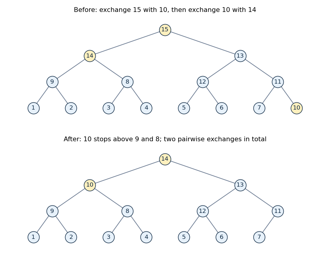
Hence the best-case maximum deletion in a binary heap is

two pairwise exchanges for n \geq 4 : one root/last exchange and one downward exchange .

(3)

This best case can be arranged at any such size: make the root child on the opposite side from the old final leaf the largest remaining key, the old leaf smaller than its own ancestors but larger than all descendants of that opposite child, and fill the remaining positions in decreasing order along each branch. The promoted child then allows the leaf to stop at depth one.

For sizes two and three, one initial exchange can suffice; for size one no exchange between distinct positions is needed. If only exchanges during heapify down are counted, the answer for

n \geq 4

is one. In the fifteen-key example the two exchanges involve three distinct keys, namely fifteen, ten and fourteen. An implementation that moves a hole by assignments need not perform literal swaps, so the count is explicitly tied to the exchange implementation. The worst-case time complexity remains logarithmic even though this best-case repair is constant.

d

Solution

Assume

1 \leq k \leq n

. Use bottom-up heap construction to make a max-heap of the first

k

input items. For each subsequent input value

x

, compare it with the root. If

x

is at least the root, discard it; otherwise replace the root by

x

and apply heapify down. Return the final root.

The loop invariant says the heap contains a multiset of the

k

smallest values seen so far. It holds after initialization. If

x

is at least the current largest retained value, the already retained

k

items are no larger, so discarding

x

preserves the invariant. If

x

is smaller, remove one largest retained value and keep

x

instead; precisely the

k

smallest values remain. This argument handles equal integers by treating repeated occurrences as separate items. At the end,

the heap root is the k th smallest input value .

Construction costs

O (k)

; each remaining value uses one comparison and at most one logarithmic repair. Thus the selection algorithm has time complexity

O (n + (n - k) lo g k) = O (n lo g k) (k \geq 2), O (k) space .

For

k = 1

, the heap is a single running minimum and the time is

O (n)

. The uniform expression

O (n lo g (k + 1))

covers that boundary; interpreting the printed

O (n lo g k)

literally at

k = 1

would incorrectly make it zero.

G = (V, E)

with undirected edges and edge weights

w

, a spanning tree is a connected, acyclic subgraph containing all vertices. It has

∣ V ∣ - 1

edges. A minimum spanning tree is one minimizing the sum of its edge weights:

T \in F \subseteq E (V, F) is a tree arg min e \in F \sum w (e) .

It minimizes total weight, rather than the distance of every route from a chosen root. Equal edge weights may permit more than one minimum spanning tree; negative weights do not invalidate the definition.

b

Solution

A precise safe-extension form of the cut lemma for minimum spanning trees is as follows. Let

F \subseteq E

be contained in some minimum spanning tree. Let

S

be a nonempty proper subset of

V

, and suppose no edge of

F

crosses the cut of a graph

(S, V ∖ S)

. If

e

is any least-weight crossing edge, then

F \cup {e} is contained in some minimum spanning tree .

To prove it, choose a minimum spanning tree

T

containing

F

. If

e \in T

, it already certifies the claim. Otherwise inserting

e

creates a graph cycle. The other part of that graph cycle must cross the cut of a graph, so choose a crossing edge

f \in T

. It does not belong to

F

, and

w (e) \leq w (f)

. Then

T - f + e

is a spanning tree containing

F \cup {e}

, of weight no greater than the optimum. It is therefore also optimal.

With

F = \emptyset

, a lightest crossing edge belongs to at least one minimum spanning tree. If that edge is uniquely lightest, it belongs to every minimum spanning tree, the strict version of the minimum spanning tree cut property. With ties, “every” would be false: in an equal-weight triangle either crossing edge can be omitted from some optimum.

c

Solution

Run Kruskal's algorithm in nonincreasing order of edge weight, accepting an edge exactly when its endpoints belong to different current connected components. Use a disjoint-set data structure to test and merge those components. Stop after accepting

∣ V ∣ - 1

edges.

Equivalently, apply ordinary Kruskal's algorithm to

w^{'} (e) = - w (e)

. For every spanning tree,

e \in T \sum w^{'} (e) = - e \in T \sum w (e),

so minimizing transformed total weight is exactly maximizing original total weight. Thus the output is a maximum spanning tree. Equal weights may be processed in any fixed order. Sorting dominates the time complexity, giving

O (∣ E ∣ lo g ∣ E ∣ + ∣ V ∣)

with the usual efficient disjoint-set data structure.

d

Solution

Build a maximum spanning tree

T

by the decreasing-weight version of Kruskal's algorithm. For the specified distinct endpoints

s, t

, find their unique graph path

P_{T}

T

by depth-first search, retaining predecessors to reconstruct it. Return that path and its minimum edge weight

b

For correctness, choose an edge

e

of weight

b

P_{T}

. Deleting it splits

T

into two connected components, separating

s

from

t

. No edge

f

across this cut of a graph can have

w (f) > b

: replacing

e

f

would give a spanning tree of greater total weight, contradicting maximality of

T

Every

s

–

t

graph path

P

must cross the same cut of a graph, so it contains a crossing edge

f

with

w (f) \leq b

. Therefore its minimum edge weight is at most

b

. The tree route attains

b

, proving

e \in P_{T} min w (e) = P : s ⇝ t max e \in P min w (e) .

This is precisely the widest path problem. The proof allows tied, zero and negative edge weights. It depends on maximizing the total tree weight, not on a shortest-distance algorithm.

Let

v = ∣ V ∣

and

e = ∣ E ∣

. Sorting and Kruskal's algorithm take

O (e lo g e + v)

time; the tree search adds

O (v)

. Hence

time O (e lo g e + v), auxiliary space O (e + v) .