Photon counting

Photon counting registers discrete detector events and their times. A beam splitter sends the selected light to two photodetectors; a coincidence circuit or time-recording system compares the outputs. With a vacuum input at the unused optical port, splitter fractions $R,T$ and independent quantum efficiencies ${\eta }_1,{\eta }_2$, a selected input photon reaches the two recorded channels with probabilities $p_1=R{\eta }_1$ and $p_2=T{\eta }_2$. Conditional on input occupation $N$, each pair of distinct photons contributes $p_1{p}_2$ to the cross-channel pair moment. ThereforeTheir normalized ratio recovers $g^{(2)}(0)$. This assumes number-resolving counts, or sufficiently dilute gates for threshold detectors to approximate them. One photon cannot create both channel counts in this ideal model.

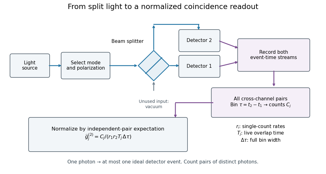
For stationary continuous detection, let $C_j$ count all cross-channel pairs with $t_2-t_1$ in a bin of full width $\Delta \tau$, and let $r_1,r_2$ be observed single-count rates. Let $T_j$ be their joint live observation time at that delay, approximately the common duration $T_{\mathrm{obs}}$ when delays are short. Independent streams have expected pair count $r_1{r}_2{T}_j\Delta \tau$, giving the displayed estimator. It estimates a bin average of second-order optical coherence, further blurred by detector timing response. For a finite uninterrupted run the exact overlap weighting is $T_{\mathrm{obs}}-|\tau |$ inside the delay integral, rather than a constant at long delays.

For an original numerical example, choose $r_1=2000{\mathrm{s}}^{-1}$, $r_2=3000{\mathrm{s}}^{-1}$, $T_j=100\mathrm{s}$, and $\Delta \tau =10\mathrm{ns}$. The independent reference is six pairs per bin. Chosen counts $C_j=3,6,12$ give estimates $0.5,1,2$; they are teaching inputs with large counting fluctuations, not historical measurements. For pulsed sources, compare properly normalized same-pulse and separate-pulse coincidences instead of assuming this continuous-source baseline.

Detector dead time suppresses nearby same-detector counts and can manufacture an apparent dip in a single-detector record. Two independent detector channels avoid that particular same-channel exclusion, but shared electronics can still reject pairs. Timing spread and wide bins wash out narrow features. A device recording only the first stop after each start measures a waiting-time distribution; interpreting it as all-pair correlations requires a sufficiently low stop probability over the relevant delay range.

Independent loss alone leaves normalized factorial moments invariant: if every input photon is retained with probability $\eta$, binomial thinning conditional on a total gives $⟨K⟩=\eta \mu$ and $⟨K(K-1)⟩={\eta }^2⟨N(N-1)⟩$. Both powers cancel from $g^{(2)}(0)$. Fewer coincidences still mean poorer statistical precision.

Now let each channel contain a signal rate $s_i$ and an independent Poisson process background rate $b_i$, independent also of the signal. Put ${\rho }_i=s_i/(s_i+b_i)$. The pair density is $s_1{s}_2{g}_{\mathrm{sig}}^{(2)}+s_1{b}_2+b_1{s}_2+b_1{b}_2$. Dividing by $(s_1+b_1)(s_2+b_2)$ proves the displayed formula, for the same bin and timing response. For chosen equal signal fractions ${\rho }_1={\rho }_2=4/5$, ideal signal values $0,1,2$ become $9/25,1,41/25$. Background pulls both dips and peaks toward one.

This calculation assumes additive, mutually independent background counts. Scattered coherent light that interferes with the signal, correlated electronic noise, or recovery effects require a different model. Correcting a dip without independently estimating the backgrounds cannot establish photon antibunching.