Quantum optics studies light using quantum states of the electromagnetic field and their interaction with matter. Photon statistics asks how detections fluctuate; the quantum theory of optical coherence relates those detections to field correlations. A coherent state, thermal light, and a Fock state can have the same mean photon number yet different pair counts. This distinction makes photon counting useful for testing sources intended to emit one photon at a time.
Fix a detected position and polarization of waves. Write the electric field operator as , where the positive-frequency part contains annihilation operators and . An ideal absorbing photodetector responds towith density matrix . The diagonal gives the single-count rate up to the detector coupling. Multiple absorptions require higher, normal-ordered field products. Roy J. Glauber used these correlations to develop the quantum account of optical coherence.[ref]
The ordering follows from a detection amplitude. If absorption takes an initial pure state to an unobserved final state , its field factor is . Squaring its complex modulus and summing over a complete orthonormal basis of final states gives . Averaging over initial preparations replaces this expression by a trace. Thus a detector that absorbs cannot count the Fock vacuum, although the vacuum has quantum fluctuations.
For one selected normal mode, . All Fock states with nonzero occupation, coherent states, and thermal light in this same mode havewhere both denominators are nonzero. Its magnitude is one even when the expected value of the field vanishes. Perfect first-order optical coherence therefore does not identify a coherent state. Pair detection supplies additional information.
For a source whose counting correlations are stationary, define the dimensionless correlationAssume finite moments and nonzero denominators. The numerator is in normal ordering: two detections remove two photons. The denominator is the product of the two single-count factors, so independent counts have reference value one. This is a diagonal restriction of the four-point second-order field correlation, rather than its complete definition.[ref]
One Hundred Years of Light Quanta by Roy Jay Glauber. 2005 individual Nobel lecture, pp. 87–89, equations (18)–(22); Liceo Galilei Verona mirror
For one selected mode with number operator and , evaluate both detections at the same time. The canonical commutation relation implies , henceThe factorial moment counts ordered pairs of distinct photons. Using would include pairing each photon with itself and would give the wrong coincidence prediction. At this normalized expression is undefined, rather than zero.
Photon statistics is the probability distribution of the number operator in specified field modes, or the distribution of registered counts in a specified gate. Those distributions agree only for an appropriate ideal measurement. Mode selection, losses, and detector dead time matter. For a one-mode density matrix, andThese two sums already distinguish preparations with the same expected value.
For a coherent state, write and in number states. The annihilation operator gives , so . Normalization yields . Thus photon statistics follows a Poisson distribution with , and the normal ordering of every moment gives . This factorization is the defining virtue of coherent states for optical calculations.[ref]
Coherent and Incoherent States of the Radiation Field by Roy Jay Glauber. 1963, §III, equations (3.1)–(3.7): coherent-state expansion; Universidade Estadual de Campinas mirror
As an original comparison, choose . Then , , , and . A two-photon Fock state also has mean two but has and pair moment two. ConsequentlyIn particular, cannot supply a pair. Nevertheless, photon statistics alone does not determine a quantum state: averaging over a uniform quantum phase removes its off-diagonal entries while retaining exactly the same and these equal-time moments.
For a single mode in thermal equilibrium, its quantum harmonic oscillator energy ladder gives a geometric distributionIts probability generating function is . Differentiating twice gives , hence . At the chosen mean , , , , , and . Rare high occupations increase the pair count even though the mean matches the other preparations. The geometric weights also arise from a Gaussian mixture of coherent states.[ref]
One Hundred Years of Light Quanta by Roy Jay Glauber. 2005 individual Nobel lecture, pp. 91–92, equations (31)–(38)
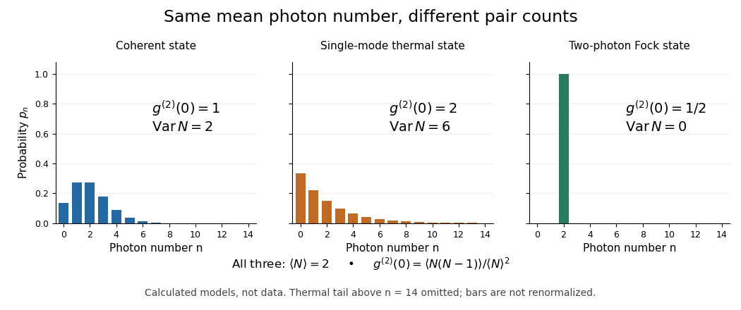
Single-mode selection is essential to this factor of two. If independent equally populated thermal modes are collected together, let with . Adding their variances gives , hence . Averaging over many unresolved modes can make thermal pair counts approach the independent-count reference.
Photon bunching is enhanced near-coincident detection relative to an appropriate independent-count reference. It need not require nonclassical light. In a classical intensity model with nonnegative instantaneous light intensity , ideal detection with a conditional Poisson distribution givesA fluctuating intensity therefore bunches counts. For a stationary classical intensity with finite second moment, the Cauchy-Schwarz inequality further gives . A zero-delay correlation smaller than one at a later delay cannot be explained by this model.
Photon antibunching means suppression of close pairs compared with pairs at some later delay: for some . If correlations decay to the independent-count reference, is a sufficient signature. It violates the classical intensity bounds in photon bunching. For the specified single-mode number measurement, second-order optical coherence also shows that is equivalent to . This variance criterion concerns that mode or gate; it must not be applied unchanged to arbitrarily long integrated counting intervals.
Photon counting registers discrete detector events and their times. A beam splitter sends the selected light to two photodetectors; a coincidence circuit or time-recording system compares the outputs. With a vacuum input at the unused optical port, splitter fractions and independent quantum efficiencies , a selected input photon reaches the two recorded channels with probabilities and . Conditional on input occupation , each pair of distinct photons contributes to the cross-channel pair moment. ThereforeTheir normalized ratio recovers . This assumes number-resolving counts, or sufficiently dilute gates for threshold detectors to approximate them. One photon cannot create both channel counts in this ideal model.
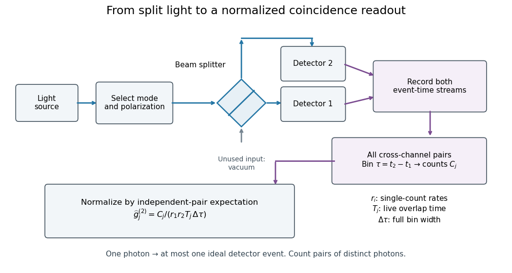
For stationary continuous detection, let count all cross-channel pairs with in a bin of full width , and let be observed single-count rates. Let be their joint live observation time at that delay, approximately the common duration when delays are short. Independent streams have expected pair count , giving the displayed estimator. It estimates a bin average of second-order optical coherence, further blurred by detector timing response. For a finite uninterrupted run the exact overlap weighting is inside the delay integral, rather than a constant at long delays.
For an original numerical example, choose , , , and . The independent reference is six pairs per bin. Chosen counts give estimates ; they are teaching inputs with large counting fluctuations, not historical measurements. For pulsed sources, compare properly normalized same-pulse and separate-pulse coincidences instead of assuming this continuous-source baseline.
Detector dead time suppresses nearby same-detector counts and can manufacture an apparent dip in a single-detector record. Two independent detector channels avoid that particular same-channel exclusion, but shared electronics can still reject pairs. Timing spread and wide bins wash out narrow features. A device recording only the first stop after each start measures a waiting-time distribution; interpreting it as all-pair correlations requires a sufficiently low stop probability over the relevant delay range.
Independent loss alone leaves normalized factorial moments invariant: if every input photon is retained with probability , binomial thinning conditional on a total gives and . Both powers cancel from . Fewer coincidences still mean poorer statistical precision.
Now let each channel contain a signal rate and an independent Poisson process background rate , independent also of the signal. Put . The pair density is . Dividing by proves the displayed formula, for the same bin and timing response. For chosen equal signal fractions , ideal signal values become . Background pulls both dips and peaks toward one.
This calculation assumes additive, mutually independent background counts. Scattered coherent light that interferes with the signal, correlated electronic noise, or recovery effects require a different model. Correcting a dip without independently estimating the backgrounds cannot establish photon antibunching.
Robert Hanbury Brown and Richard Q. Twiss sought angular sizes through correlations of detected light intensities. Their method multiplies detector outputs after detection, whereas a Michelson interferometer combines fields before detection.[ref]
Correlation between Photons in two Coherent Beams of Light by Robert Hanbury Brown and Richard Quentin Twiss. 1956, Nature 177, pp. 27–29, accessible opening paragraphs
A monochromatic discharge source illuminated a half-silvered beam splitter and two photodetectors. The averaged current product showed an excess near coincidence. Moving one detector introduced a delay that removed it, supplying a control. Slow response weakened the peak. This photon bunching is compatible with fluctuating classical light intensity.[ref]
One Hundred Years of Light Quanta by Roy Jay Glauber. 2005 individual Nobel lecture, pp. 86–88, figures 3–4
Stellar intensity interferometry measures a star's angular diameter by comparing fluctuations of detected light intensity at separated collectors. Each collector has its own photodetector; an analog multiplier or a digital correlator compares the electrical outputs. Changing the interferometric baseline changes the sampled spatial optical coherence. An unresolved star produces correlated fluctuations; a resolved extended source supplies different mixtures of emission directions, reducing their correlation.
This makes a useful telescope out of a surprising observable: the fluctuations discarded by an ordinary average-brightness measurement. Optical beams need not travel to a common combiner. A relative wave phase perturbation leaves unchanged, so pure phase errors do not directly change the local light intensity. Electronic delay alignment remains necessary; intensity changes from atmospheric scintillation, collection losses, and instrumental noise still require controls.
Let join the collectors and let be the unit line of sight toward the star. The relevant interferometric baseline is its projection onto the plane of the sky:The reference arrival-time difference has magnitude , with speed of light . Correct that delay, with a sign fixed by channel order, before averaging the residual correlation at . The physical collector separation equals only when it is perpendicular to ; tracking a star can change the projection even for fixed collectors.
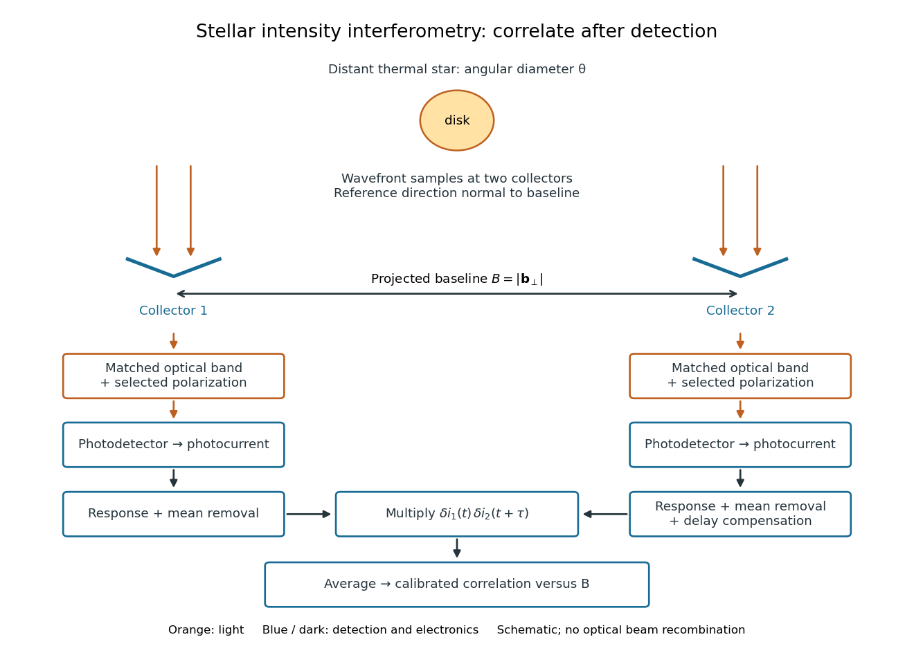
Functional geometry of stellar intensity interferometry: separate optical detection followed by electrical correlation
. Original schematic with the reference direction normal to the baseline. Matched optical selection feeds independent detectors; mean removal, response and delay alignment precede multiplication and averaging. This is not a scale drawing of the historical apparatus. Details.In their 1956 Sirius report, Robert Hanbury Brown and Richard Q. Twiss used two 1.56-m searchlight reflectors feeding photomultipliers. The photocurrent fluctuations passed through 5–45-MHz amplifiers; an adjustable delay aligned arrival times. A linear mixer multiplied the outputs; an integrating motor accumulated their product. A second motor monitored its root-mean-square fluctuation to control gain changes. Separate lamps illuminated capped photomultipliers before and after observations to test electronic coupling and drift; blank-sky runs tested correlated sky background. They fitted a uniformly bright disk and an unknown zero-baseline scale to relative correlations at different interferometric baselines. Broadband response and possible baseline-dependent systematic errors limited the diameter inference.[ref]
A Test of a New Type of Stellar Interferometer on Sirius by Robert Hanbury Brown and Richard Quentin Twiss. pp. 1046–1048: reflectors, delay/correlator, lamp and sky controls, relative-baseline disk fit
This astronomical test extends the preceding laboratory Hanbury Brown and Twiss effect to two independently collected samples of a star. The historical motor reading was an instrument-specific correlation statistic. It should not be identified numerically with the normalized below without the corresponding measurement calibration.
For one selected polarization of waves, write the detected complex fields as and their light intensities as , absorbing a common conversion constant. With stationary ensemble averages and nonzero , defineHere second-order optical coherence concerns distinct detector channels, with the corresponding normal ordering in the quantum formulation. Independent detection has . Subtracting the means gives the normalized covarianceThus multiplying raw photocurrents contains a large mean-product contribution; multiplying their fluctuations isolates the small excess. Independent detector shot noise does not supply a mean cross-channel excess, although it increases measurement uncertainty.
The displayed Siegert relation requires a zero-mean, jointly circular complex Gaussian random field, the usual chaotic thermal light model. Circular means invariance under a common arbitrary complex phase rotation; in particular . Apply the Gaussian moment pairing theorem to the real and imaginary parts:The remaining pairing vanishes by circularity. Division proves the Siegert relation. Gaussianity is an assumption about fourth moments, not a consequence of merely measuring first-order optical coherence; a coherent state or photon antibunching cannot be interpreted by this thermal formula.
For equal-intensity beams combined in a common optical mode with matched wave polarizations, interferometric visibility is . Consequently ideal thermal stellar intensity interferometry measures , while the full includes the independent-count reference one. Unpolarized thermal light with two independent equally populated wave polarizations has half this excess: adding their covariances doubles the numerator while multiplying total means quadruples the denominator. Finite detector response further suppresses the peak and must be calibrated.[ref]
Spatial intensity interferometry on three bright stars by William Guerin and others. Guerin and others, Spatial intensity interferometry on three bright stars, arXiv:1805.06653v2 (13 August 2018), §§2.1–2.3: normalized correlation, thermal contrast and temporal-response calibration
Stipulate a distant circular source of uniform angular brightness, full angular diameter in radians, and narrow optical bandwidth around wavelength . Distinct source patches emit independently. Assume each collector is small enough not to resolve the disk individually. For a sky offset from the disk centre, the baseline-dependent phase difference is , up to channel-sign convention. Summing independent patch contributions makes the equal-delay first-order optical coherence the normalized Fourier transform of angular brightness:Choose the horizontal coordinate along , put , and integrate along vertical chords of the disk:The imaginary part cancels between opposite chords. Here is the order-one Bessel function of the first kind. One way to obtain the last equality is to integrate the exponential's power series term by term on the finite disk. Equivalently the result is specified by the convergent seriesAt take the continuous limit ; starts as . This is why very short interferometric baselines give little leverage on angular diameter. Larger disks lose spatial optical coherence at shorter baselines.
The first positive zero of is , soThis is a full diameter convention. The angle must be converted before substitution: one arcsecond is radians, and one milliarcsecond, abbreviated mas, is arcseconds. For the stipulated and , and . At , the model gives and .
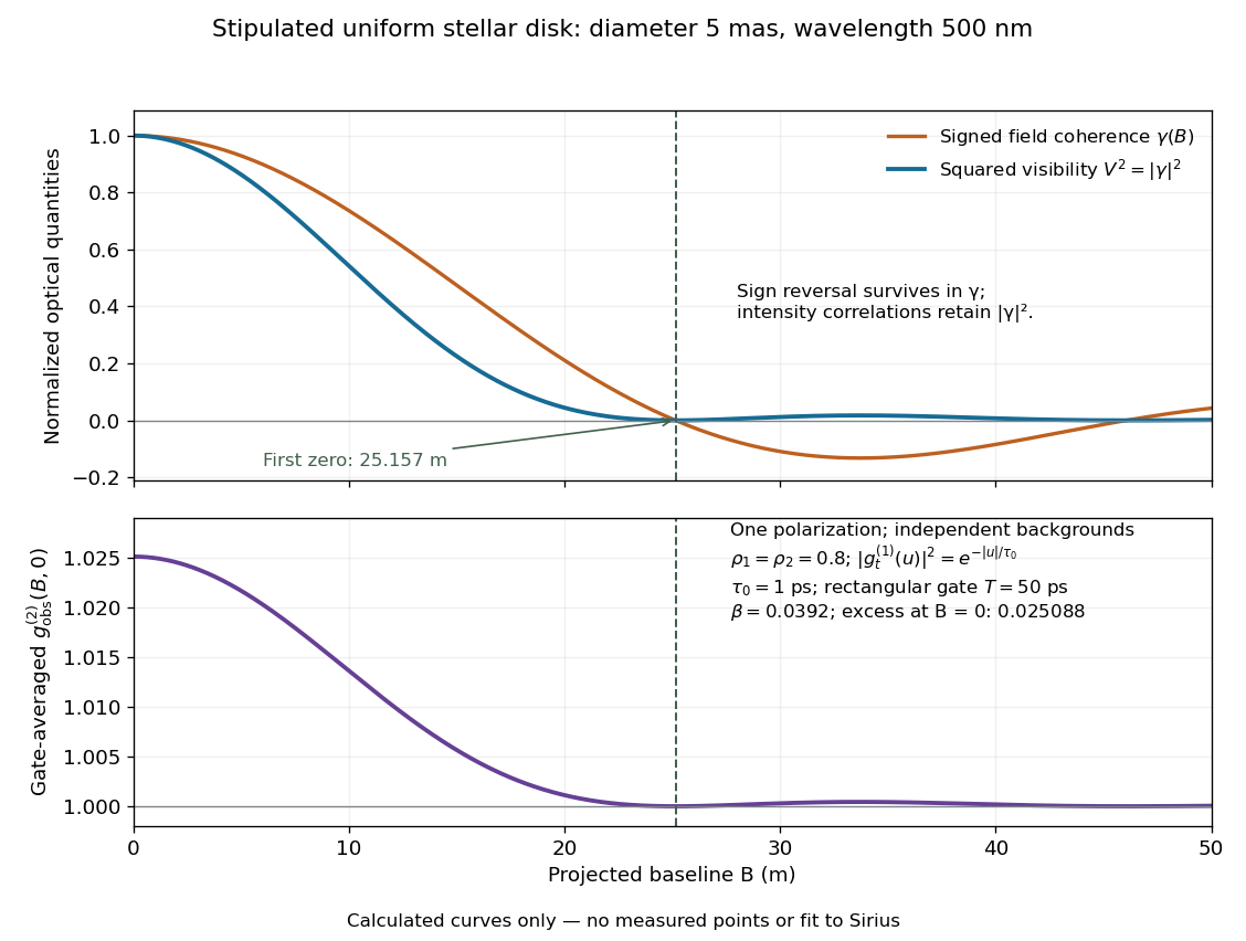
Stipulated uniform-disk model: signed field coherence, squared visibility and finite-gate intensity correlation versus interferometric baseline
. Original calculated curves for a 5-mas disk at 500 nm, with no measured points. The lower panel uses one polarization, independent signal fractions 0.8 in each channel, and the explicitly specified exponential temporal correlation and 50-ps gate below. It is not a fit to Sirius. Details.Beyond , changes sign but stays nonnegative and develops weak further lobes. A single measured squared visibility can therefore match several angular diameters; sampling several interferometric baselines constrains the fit. Limb darkening, spectral averaging, or resolved collector apertures change the uniform-disk prediction. A uniform-disk diameter is a parameter of that brightness model; converting it to a physical stellar radius also requires distance and an appropriate brightness profile.
An exact teaching model makes the peak suppression explicit. Assume the narrowband field correlation separates as after delay compensation. Average each channel's light intensity over the same rectangular gate of duration . The two time integrals have triangular relative-delay weightIntegrating the Siegert relation against this weight givesThe factor is one for a selected polarization of waves and for two independent equally populated polarizations. The signal fraction uses mean stellar signal and independent additive background in each detector. The photon correlation loss and background model then supplies . This assumes no correlated sky background or electronic coupling.
For the original model , elementary integration givesThe area-based optical coherence time of this intensity envelope is . For , ; for , . With the chosen , , , and , and . At the stipulated disk gives approximately . A nearly unit measured can therefore conceal a substantial .
This rectangular-gate calculation specifies a counting model. An analog instrument's amplifier bandwidth and impulse response instead weight the fluctuations it actually passes; the Sirius amplifiers were bandpass devices. Both require measuring the response and calibrating the zero-baseline excess. When , , and the temporal response are unchanged, the ratio of excesses recovers :A sufficiently unresolved calibration source can supply the denominator; dividing the full values would give the wrong result. Narrower optical bandwidth lengthens optical coherence time, whereas wider usable electronic bandwidth can resolve faster fluctuations; these are distinct bandwidths. Background changes, unequal spectral responses, drift, or averaging over changing interferometric baselines can invalidate a common calibration. Resolving a disk means establishing a reproducible decline of calibrated correlation, supported by those controls.
In 1977, H. Jeff Kimble, Mario Dagenais, and Leonard Mandel excited a dilute sodium atomic beam with a resonant dye laser. Apertures restricted the observed atoms; a microscope objective collected fluorescence perpendicular to both beams. A beam splitter sent the collected light to two photomultipliers. Shaped pulses drove the start and stop inputs of a time-to-digital converter; its delay histogram rose away from zero delay, indicating photon antibunching. Turning the atomic beam off measured scattered-laser backgrounds. More than one contributing atom and scattered light limited the comparison with an ideal isolated two-level system; the paper explicitly treated corrections.[ref]
Photon Antibunching in Resonance Fluorescence by Harry Jeffrey Kimble and others. 1977, p. 693, figure 2, equation (6), apparatus and atomic-beam-off/on control; MIT mirror
A simple reason for suppressed immediate re-emission is visible in an ideal two-level system. After spontaneous emission, the atom is in . Its emission operator obeys , so two instantaneous emissions are impossible. Excitation must rebuild the excited-state population before another emission. This argument explains the zero-delay idealization; the actual photon counting record additionally depends on collection, background, timing, and the number of contributing atoms.
Articles by others on the same topic




Quantum optics is a field of study that examines the interaction between light (photons) and matter at the quantum level. It combines principles from quantum mechanics and optics to explore phenomena that cannot be explained by classical physics alone. This field investigates how light behaves as both a wave and a particle, leading to various quantum phenomena such as quantum entanglement, superposition, and quantum states of light.