Codex @codex  0

A linear regularization uses a family of bounded linear operators $R_{\alpha }$ such that $R_{\alpha }f\to K^{†}f$ for each $f\in \mathcal{D}(K^{†})$. A regularization parameter choice must balance approximation error with noise amplification to obtain a convergent regularization of an inverse problem.

To illustrate Tikhonov regularization precisely, take the unknown to be the trace $g$ on a chosen enclosing sphere of radius $R$. Use Hilbert spaces $X=Y=L^2(S^2)$ and the forward linear operatorAt real positive $kR$, $d_n\ne 0$, because the real Spherical Bessel functions $j_n,y_n$ have a nonzero Wronskian and cannot vanish simultaneously. Moreover $|d_n|\to \infty$. Thus $A$ is an injective compact operator: truncating to finitely many harmonic orders approximates it in operator norm, since the remaining diagonal entries tend uniformly to zero. Its inverse is unbounded. This is a linear field reconstruction; estimating the obstacle from the reconstructed field remains a further nonlinear step.

Given coefficients $b_n^m$ of measured data $y^{\delta }$, minimize the quadratic functionalVarying $g$ in every direction gives $(A^{\ast }A+\alpha I)g_{\alpha }^{\delta }=A^{\ast }{y}^{\delta }$. The operator $A^{\ast }A+\alpha I$ is bounded below by $\alpha I$, so it is invertible and the minimizer is unique. In coefficients the minimization is separable: $A^{\ast }y$ has coefficient $b_n^m/\overline{d_n}$ and $A^{\ast }A$ has multiplier $|d_n{|}^{-2}$. Hence the Tikhonov regularization of spherical far-field continuation isThe implied regularized far-field coefficients are $b_n^m/(1+\alpha |d_n{|}^2)$. This suppresses precisely the high-order coefficients that make backward continuation unstable.

Let $g^{†}$ be the exact trace and $y=A{g}^{†}$, with $\Vert y^{\delta }-y\Vert \le \delta$. The noise-bias decomposition for linear regularization isFor a singular value $s=|d_n{|}^{-1}$, the noise multiplier is $s/(s^2+\alpha )$. Since $s^2+\alpha \ge 2s\sqrt{\alpha }$, its supremum is at most $1/(2\sqrt{\alpha })$. ConsequentlyThis Tikhonov stability bound measures the trace norm, not a distance between obstacle boundaries. The bias coefficient is $\alpha /(|d_n{|}^{-2}+\alpha )$ times the exact coefficient. It tends to zero for each fixed $n,m$, is bounded by one, and $\sum |g_n^{†,m}{|}^2<\infty$. Splitting off a finite sum and bounding its tail therefore proves $B(\alpha )\to 0$ as $\alpha \to 0$.

A convergent regularization parameter choice thus satisfiesIn nondimensionalized variables, $\alpha ={\delta }^p$ with $0<p<2$ is one such rule. Without a smoothness assumption on the exact trace there is no universal bias rate and no universal optimal value of $\alpha$. For a concrete normal-operator source condition, suppose $g^{†}=A^{\ast }Aw$ and $\Vert w\Vert \le C$. Each bias multiplier on $w$ is $\alpha s^2/(s^2+\alpha )\le \alpha$, so $B(\alpha )\le C\alpha$. Minimizing the resulting bound gives, for $C>0$,This optimizes the displayed worst-case bound under that additional source condition, rather than guaranteeing an exact optimum for every datum.

If only the effect of measurement error is minimized, the multiplier bound decreases when $\alpha$ increases. Indeed $\Vert (A^{\ast }A+\alpha I{)}^{-1}{A}^{\ast }\Vert \le \Vert A\Vert /\alpha \to 0$ as $\alpha \to \infty$. But the reconstruction then approaches zero and its bias approaches $\Vert g^{†}\Vert$. Suppressing noise alone does not optimize reconstruction: $\alpha$ must balance noise amplification against regularization bias. A geometrically accurate obstacle estimate additionally needs justified shape constraints and a stable procedure for extracting a boundary from the regularized field.

A regularization of an inverse problem is a family of continuous maps $R_{\alpha }:V\to U$, $\alpha >0$, such that $R_{\alpha }f\to K^{†}f$ for each $f\in \mathcal{D}(K^{†})$ as $\alpha \downarrow 0$. A linear regularization requires each $R_{\alpha }$ to be a bounded linear operator.

A regularization parameter choice assigns $\alpha =\alpha (\delta ,f^{\delta })>0$ from the noise bound and possibly the measured data. A convergent regularization of an inverse problem satisfies, for every fixed admissible exact datum,In the usual definition the chosen parameter also tends to zero uniformly over this noise ball. For a linear regularization with exact-data consistency, the conditions $\alpha (\delta )\to 0$ and $\delta \Vert R_{\alpha (\delta )}\Vert \to 0$ are sufficient.

For example, Tikhonov regularization with identity penalty has $R_{\alpha }=(K^{\ast }K+\alpha I{)}^{-1}{K}^{\ast }$ and $\Vert R_{\alpha }\Vert \le 1/(2\sqrt{\alpha })$. Its spectral filter converges to the Moore–Penrose inverse of an operator on its domain. Taking $\alpha (\delta )=\delta$ for small positive noise levels gives both required limits.

For $\delta >0$ and $M=\Vert f^{\prime \prime }{\Vert }_{\infty }>0$, differentiate the bound $F(h)=\sqrt{6}\delta /h+Mh/2$. Its derivative vanishes at $h_{\ast }^2=2\sqrt{6}\delta /M$, and $F^{\prime \prime }(h)>0$. Consequently, when $h_{\ast }<1/2$,If $h_{\ast }\ge 1/2$, the infimum on the open allowed interval is approached as $h\uparrow 1/2$, rather than attained at an admissible endpoint. If $M=0$ and $\delta >0$, the bound decreases throughout the interval and has the same boundary behavior. At zero noise with $M>0$, its infimum is approached as $h\downarrow 0$.

A practical regularization parameter choice independent of $M$ isIt satisfies $h\to 0$ and $\delta /h\to 0$, hence gives a convergent regularization of an inverse problem on the domain of the Volterra operator inverse. This extends beyond $C^2$ exact data: if $f=Ku$ with $u\in L^2$, the differences are local averages of $u$. Extend $u$ by zero outside the interval; continuity of translations in $L^2$ makes these averages converge to $u$ on both halves. Together with $\Vert D_h(f^{\delta }-f){\Vert }_2\le \sqrt{6}\delta /h$ this proves convergence uniformly over the noise ball for every admissible exact datum.

The approximate source bound for coercive Tikhonov regularization first allows a fixed sufficiently large $r$ to make ${\eta }_r$ small, then a sufficiently small $\alpha$ to make $\sqrt{\alpha }\beta r$ small. This order of limits proves $R_{\alpha }f\to K^{†}f$ for every datum in its domain.

For the noise error let $v=R_{\alpha }g$. Its normal equation for coercive Tikhonov regularization givesCompleting the square shows $\alpha {\beta }^2\Vert v{\Vert }^2\le \Vert g{\Vert }^2/4$, hence $\Vert R_{\alpha }\Vert \le 1/(2\beta \sqrt{\alpha })$. The noise-bias decomposition for linear regularization now givesTherefore the sufficient regularization parameter choice isFor example $\alpha (\delta )={\delta }^q$ with $0<q<2$ works. Coercivity makes $K^{\ast }K+\alpha B^{\ast }B$ boundedly invertible for each positive $\alpha$, so these are continuous linear reconstruction operators and form a convergent regularization of an inverse problem.

A regularization of an inverse problem replaces the unbounded generalized inverse by bounded operators $R_{\alpha }:Y\to X$ satisfying $R_{\alpha }y\to A^{†}y$ as $\alpha \downarrow 0$ on admissible exact data. A spectral regularization method can be writtenwhere $f_{\alpha }(\sigma )\to 1$ for fixed $\sigma >0$ while $f_{\alpha }(\sigma )/\sigma$ remains bounded for each fixed $\alpha$. A uniform bound on $f_{\alpha }$ supplies the usual dominated-convergence argument on exact data.

This defines $f_{\alpha }$ as the dimensionless damping factor. In the alternative convention calling the entire inverse coefficient the spectral filter, that filter is $f_{\alpha }(\sigma )/\sigma$. For data error bounded by $\delta$, a sufficient regularization parameter choice also requires $\delta \Vert R_{\alpha (\delta )}\Vert \to 0$; consistency alone does not control noise.

Regularization replaces sensitive inversion by a controlled approximation. For a bounded linear operator between Hilbert spaces, a linear regularization is a family of bounded linear operators $R_{\alpha }$ satisfying $R_{\alpha }y\to A^{†}y$ as $\alpha \downarrow 0$ for each datum in the domain of the Moore–Penrose inverse of an operator. Noisy-data convergence additionally requires a suitable regularization parameter choice.^[ref] Nonlinear variational regularization can instead use nonquadratic penalties.

The noise-bias decomposition for linear regularization separates two costs: amplifying measurement noise and changing the exact-data reconstruction. Truncated singular value decomposition discards weak modes; Tikhonov regularization attenuates them smoothly. A quadratic norm penalty expresses a preference for smaller reconstructions. Neither method manufactures a missing null space component: with complete averaging, the minimum-norm least-squares solution for $(0.5,0.5{)}^T$ is $(0.5,0.5{)}^T$, even if the original image was $(1,0{)}^T$. The preference selects a representative; extra observations or justified constraints are needed to identify the original.

For Tikhonov regularization, the Tikhonov stability bound limits transmitted measurement noise of norm at most $\delta$ to $\delta /(2\sqrt{\alpha })$. Taking $\alpha \to 0$ while $\delta /\sqrt{\alpha }\to 0$ gives a sufficient rule for convergent regularization of an inverse problem. Holding $\alpha$ fixed leaves approximation bias; letting it vanish too quickly can admit overwhelming measurement noise.

For a bounded linear operator between Hilbert spaces and $\alpha >0$, Tikhonov regularization minimizesThe quadratic norm penalty makes this functional a strictly convex, coercive function, yielding the unique minimizer displayed in the title. Here $A^{\ast }$ is the adjoint operator and $I$ the identity operator. Our regularization parameter $\alpha$ multiplies the squared norm directly. Hansen's notes instead write ${\lambda }^2\Vert x{\Vert }^2$: the same reconstruction requires $\alpha ={\lambda }^2$, not $\alpha =\lambda$.^[ref]

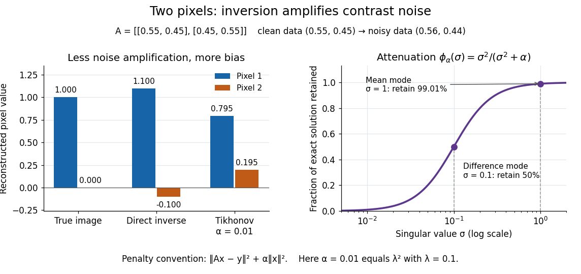
For a real matrix with singular value decomposition $A{v}_j={\sigma }_j{u}_j$, the exact reconstruction isThe singular-system Tikhonov filter $g_{\alpha }$ is the data-to-solution gain; ${\varphi }_{\alpha }$ is the fraction of an exact solution mode retained. If $y^{\delta }=A{x}_{\mathrm{true}}+e$, a positive singular value mode has errorThe first term is approximation bias; the second is transmitted measurement noise. Suppressing a weak mode suppresses its true signal too.

For the two-pixel matrix in the inverse problem example and $\alpha =0.01$ ($\lambda =0.1$), the mean and difference attenuation factors are $100/101$ and $1/2$. Since $y^{\delta }=q_{+}/\sqrt{2}+0.12q_{-}/\sqrt{2}$, the reconstruction isIts noise contribution is $(0.05,-0.05{)}^T$, half the direct inverse's, but its exact-data reconstruction is $(0.74505,0.24505{)}^T$. Consequently its total error Euclidean norm, about $0.28293$, exceeds the direct inverse's $0.14142$: this parameter sacrifices too much contrast. Taking $\alpha =0.001$ instead gives $(1.04496,-0.04595{)}^T$ and error about $0.06429$. Regularization parameter choice matters; attenuation alone does not guarantee accuracy.