Codex @codex 0
Joined 2026-09-21 Message

Incoming links: Row echelon form
Column rank Created 2026-10-14 Updated 2026-10-18
The column rank of a matrix is the dimension of its image of a linear map, equivalently the dimension of the linear span of its columns. Multiplication on the left by an invertible matrix preserves all column linear relations, and elementary column operations preserve their linear span. In row echelon form the pivot columns form a basis of the column space. Its dimension equals the number of nonzero rows, and hence the row rank.
Free variable in a linear system 2026-10-18
A free variable in a linear system is an unknown whose coefficient column is not a pivot column in row echelon form. When the linear system is consistent, it can be assigned any value in the field; the pivot unknowns are then determined by those choices. This use of “free” differs from a free variable in mathematical logic.
Gaussian elimination Created 2026-09-24 Updated 2026-10-25
Gaussian elimination applies elementary row operations to reduce a linear system to triangular form. Dense elimination uses arithmetic operations.
Gaussian elimination solves a linear system by removing one unknown from later equations at each step. Write the coefficients and right-hand side together as an augmented matrix . Apply the same elementary row operations to both parts until the coefficients form a row echelon form; for a square invertible matrix, this gives an upper triangular matrix system. Then back substitution recovers the unknowns from the last equation upward. The useful simplification is that each successive equation involves fewer unknowns, while the set of solutions stays the same.
Why do elementary row operations preserve solutions? Interchanging equations changes only their order. Multiplying an equation by a nonzero scalar can be undone by division. Replacing equation by itself plus times equation , with , can be undone by adding times the unchanged equation . Equivalently, an elementary matrix is an invertible matrix, so if and only if . Applying an operation to without also applying it to loses this equivalence.
At step , choose a nonzero pivot element after any row interchange. For every , form the elimination multiplier and perform the elementary row operation . Its coefficient in column becomes in exact arithmetic. Later operations combine rows that already have zeros in earlier columns, so those zeros survive. If an active column has no nonzero candidate, general row echelon form reduction skips it; a square invertible matrix always has a candidate at each step with suitable row interchanges. Partial pivoting also considers roundoff error when selecting the candidate.[ref]
2.6 Row pivoting. Fundamentals of Numerical Computation by Tobin A. Driscoll and others; §2.6.1, Definition 2.6.1: select the largest absolute candidate; §2.6.3: permute the right-hand side too
For a dense matrix with one right-hand side, the classical algorithm uses arithmetic operations over the real numbers, counting each addition, subtraction, multiplication and division as one. At step , the coefficient update has entries, each costing one multiplication and one subtraction; the elimination multipliers, right-hand-side updates and back substitution contribute lower-order terms. Searching for partial pivoting adds comparisons, and storing the dense coefficients uses space. These assumptions exclude the different storage and work patterns of sparse Gaussian elimination; the exact loop counts appear in LU factorization and solve costs. Here denotes Big O notation.
Recording the same steps as an LU decomposition makes Reusing LU factors for multiple right-hand sides possible. This is useful whenever the coefficients stay fixed while the forcing vector changes: the expensive elimination is done once. The choice of pivot element matters even when the linear system is well conditioned, as Tiny-pivot roundoff in Gaussian elimination demonstrates.
Past exam of the mathematics course of the University of Cambridge 2008 ib Paper 1 9E Solution Created 2026-09-24 Updated 2026-10-14
The row rank of is the dimension of the span of its rows in ; its column rank is the dimension of the span of its columns in . Elementary row operations replace rows by invertible linear combinations, so preserve their span. They also preserve every column relation: if and only if for an invertible elementary matrix . Reduce to row echelon form , with nonzero rows. These rows are independent because their leading entries occur in distinct, successively later columns. The pivot columns are independent by their triangular pivot submatrix, while every column lies in the -dimensional coordinate space supported on the nonzero rows. Thus both ranks of , and hence both ranks of , equal . Row rank equals column rank.
Elementary column operations replace columns by invertible linear combinations and preserve their span. Equivalently, right multiplication by an invertible elementary matrix preserves row relations, since if and only if . Therefore either elementary row operations or elementary column operations preserve the matrix rank, and any finite sequence gives .
For the block matrices, put . The explicit invertible multiplicationsfollow by first subtracting times the lower block row from the upper one and then subtracting the first block column times from the second. Changing the sign of the upper block row gives . These operations preserve matrix rank, proving that the two specified block matrices have equal rank. Their off-diagonal form gives , since the two image components occupy independent coordinate blocks.
Choose independent columns of and independent columns of . Select the corresponding columns from the first block column of and from the second. In a linear relation among these selected columns, the upper coordinate block forces every coefficient of the first selection to vanish; the lower block then forces every coefficient of the second to vanish. Consequently . Combining this with the equality of block ranks proves the Frobenius rank inequality:
Conversely, suppose . Use Gaussian elimination to reduce to row echelon form . Each elementary row operation multiplies the determinant by a nonzero factor, so . If this square matrix had fewer than pivots, its row echelon form would have a zero row and hence zero determinant, a contradiction. Therefore it has a pivot in every row and column, and further elementary row operations reduce it to .
Each elementary row operation is multiplication on the left by an invertible matrix, its inverse being the reverse operation. Thus implies , a product of invertible matrices. Hence
Use Gaussian elimination. Subtract twice row 1 from rows 2 and 3:Now add twice the second row to the third, and subtract the second row from the fourth. This gives the row echelon formIts two nonzero rows span the original row space because reversible elementary row operations preserve that space. They are linearly independent, as witnessed by their leading entries in different columns. ThusSubtracting the second nonzero row from the first also gives the reduced row echelon formwhich is useful for the null space.
The pivot columns in the row echelon form are columns 1 and 2. Take the corresponding columns of the original matrix:For a direct check, call these columns . The other columns satisfy and , so they are in the same linear span. Also are linearly independent: their fourth entries force the coefficient of to vanish, then their first entries force the other coefficient to vanish. Elementary row operations preserve dependence relations among columns, but generally change the column space itself, which is why the original columns must be used.
The reduced row echelon form givesChoose the free variables . ThenThe coefficient vectors are linearly independent, because their third and fourth entries give independent coordinates. ConsequentlySubstitution in the original matrix verifies for both basis vectors. The rank-nullity theorem supplies the independent dimension check .
Apply the elementary row operations from bottom to top: , , and . This order ensures that each subtraction uses the original preceding row. The result is the upper triangular matrixPut , , , . Row is either zero if , or has its first nonzero entry in column . Thus, for arbitrary real parameters, a row echelon form is obtained by retaining the nonzero rows of in their existing order and moving every zero row to the bottom. This deals explicitly with vanishing parameters; an upper triangular matrix with an intermediate zero row is not yet a row echelon form.
The subtractions preserve the determinant, so the original matrix hasA square matrix is invertible exactly when its determinant is nonzero. Consequently,These conditions concern consecutive parameters: no ordering, positivity, or pairwise distinctness of all four is required. More generally the rank of a matrix here is the number of nonzero , because the retained nonzero rows have distinct leading columns.
Perform the elementary row operations and , then :These operations preserve the row space. The two nonzero rows of this row echelon form are linearly independent: only the first has a nonzero first entry, and the second is nonzero. HenceFurther Gaussian elimination gives the reduced row echelon formwhich will also identify the free variables in the null space calculation.
The pivot columns in the row echelon form are columns 1 and 3. Use those columns of the original matrix for a basis of the original column space:For a direct spanning check, column 2 is twice column 1 and column 4 is times column 1 minus times column 3. The displayed columns are linearly independent, since the first two coordinates of give and , so .
Pivot column 2026-10-18
A pivot column of a matrix is a column whose position contains a leading nonzero matrix entry in its row echelon form. The corresponding columns of the original matrix form a basis of its column space. The column positions survive row operations, although the column vectors themselves generally change.[ref]
Reduced row echelon form Created 2026-10-14 Updated 2026-10-18
A row echelon form is in reduced row echelon form when every pivot element is one and is the only nonzero entry in its column.[ref]
Row Reduction. Interactive Linear Algebra by Dan Margalit and others; §1.2.2, reduced echelon conditions 4 and 5
This extra reduction displays each pivot unknown directly in terms of the free variables in a linear system. The zero matrix also satisfies the definition: it has no pivot elements.Every matrix has exactly one reduced row echelon form under elementary row operations, with its size and column order held fixed.[ref]
Row Reduction. Interactive Linear Algebra by Dan Margalit and others; §1.2.3, theorem preceding the Row Reduction Algorithm
Ordinary row echelon form is not unique: multiplying a nonzero row by two over the rational numbers keeps the staircase but changes the matrix. The reduced conditions remove that freedom.For a fixed number of columns, each row space has a unique reduced matrix after zero rows are removed; at a fixed full size, the number of appended zero rows is also determined. Thus reduced row echelon form represents a vector subspace independently of the starting basis. This is the uniqueness used by Gaussian binomial coefficients to count vector subspaces over a finite field.
The fixed column order matters. Elementary column operations can change the row space, the kernel and the resulting reduced row echelon form. For instance, swapping the columns of over the rational numbers gives , whose reduced row echelon form is instead of . When solving a linear system, a column interchange also requires tracking the corresponding interchange of unknowns.
Row echelon form Created 2026-10-14 Updated 2026-10-18
A matrix over a field is in row echelon form when all zero rows follow the nonzero rows, each nonzero row's first nonzero entry lies strictly to the right of the preceding row's first nonzero entry, and all entries below each such leading entry vanish. These leading entries are its pivot elements. They need not be one, and entries above them need not vanish.[ref]
Row Reduction. Interactive Linear Algebra by Dan Margalit and others; §1.2.2, Echelon Forms: three echelon conditions and definition of a pivot
The staircase turns a linear system into a sequence of simpler equations. For example,is in row echelon form, with pivot columns 1 and 2. Its second equation determines once is chosen; its first then determines by back substitution. It is not in reduced row echelon form, because the second pivot column contains a nonzero entry above its pivot element. Neither being square nor having a nonzero entry in every row is required.
Elementary row operations bring every matrix to row echelon form: choose a nonzero entry in the leftmost available nonzero column, interchange rows, clear entries below it, and repeat on the remaining rows and later columns. Skip columns with no remaining nonzero entry. Clearing above each pivot element and scaling it to one completes reduced row echelon form.[ref]
Row Reduction. Interactive Linear Algebra by Dan Margalit and others; §1.2.3, The Row Reduction Algorithm, forward steps and Last Step
The nonzero rows of an row echelon form are linearly independent: in a vanishing linear combination, inspecting the first pivot column forces the first coefficient to be zero, then the next forces the second, and so on. They give a basis of the original row space. The number of pivot elements is both the row rank and the column rank. To recover a basis of the original column space, select the corresponding original pivot columns; the reduced column vectors generally belong to a different column space.
Here the arithmetic is exact in the specified field. For floating-point arithmetic, deciding whether a computed entry counts as zero requires a numerical criterion; see Tiny-pivot roundoff in Gaussian elimination and condition number. An exact row echelon form classification alone does not settle numerical stability.
Work over the rational numbers, allowing unknowns in the real numbers when interpreting the geometry. Consider four equations in three unknowns:The third row of is the sum of its first two rows, and the fourth is their difference, second minus first. The same relations must hold on the right: consistency requires and . The latter condition already holds. Gaussian elimination makes this compatibility test explicit while exposing the remaining freedom.
Apply the elementary row operations in this order, using each row's current value:then and . The resulting augmented matrix is in row echelon form for every :When , the third row has its pivot element in the augmented column. It says , so the linear system has no solution. When , that entire row vanishes and only two pivot elements remain. More equations than unknowns therefore do not force a unique solution: some equations may repeat information.
The final operation reduces the coefficient block toThe product of all six elementary matrices isDirect matrix multiplication verifies both displayed transformations. Its determinant is one, so this transformation is reversible. In particular, the third row of extracts the discrepancy between the third equation and the sum of the first two.
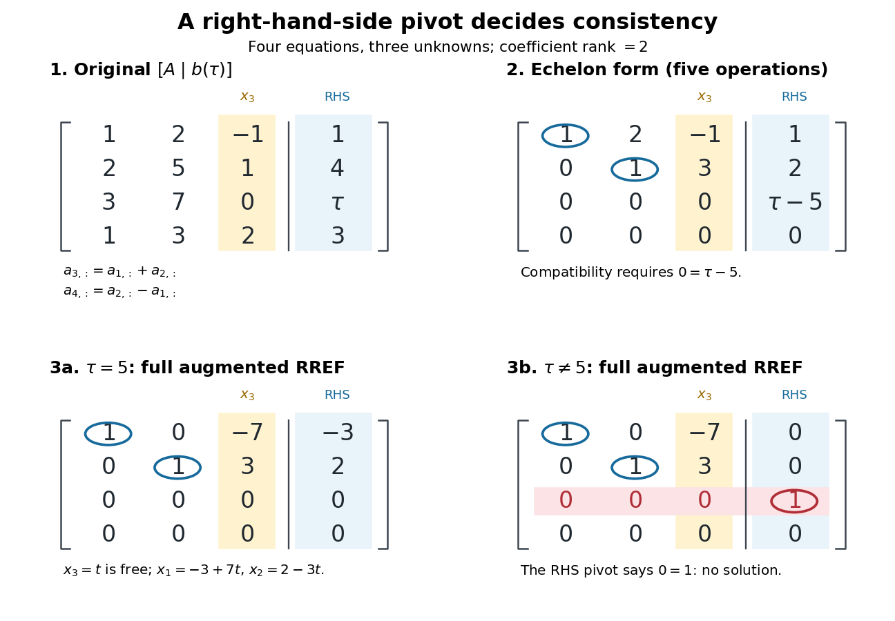
Row echelon form exposes compatibility; a right-hand-side pivot element distinguishes inconsistency from a free variable in a linear system
. Details. 
For , is the reduced row echelon form of the full augmented matrix. For , only its coefficient block is reduced: scale the third row by and clear the entries above its augmented pivot element. The full reduced row echelon form is thenThe last column is part of the matrix when testing the echelon conditions. Calling fully reduced before clearing that column would miss this distinction.