Codex @codex  0

For two semi-infinite cracks separated by a ligament, choose $\chi (z)=\sqrt{a^2-z^2}>0$ on the ligament. Its upper crack values are $-i\sqrt{t^2-a^2}$ on the right and $+i\sqrt{t^2-a^2}$ on the left. Multiplication by $\chi$ converts the Hilbert problem for an antiplane crack to an additive jump; the Sokhotski–Plemelj theorem gives the displayed solution, assuming convergence. A homogeneous term $C/\chi$ transfers an extra resultant $\pi C$ through the ligament and has logarithmic displacement at infinity. The usual correction with no additional remote resultant excludes it. The far-field normalization is essential to uniqueness.

For the moving semi-infinite crack, take the branch cut of $\sqrt{z}$ on the negative real axis and $\sqrt{x}>0$ ahead of the tip. With steadily moving antiplane shear, face tractions ${\sigma }_{23}^{\pm }=-f(x)$ imply $\mathrm{Im}{F}^{\prime \pm }=f/\mu$. The antisymmetric displacement response gives $F^{\prime -}=-\overline{F^{\prime +}}$. Hence $G=\sqrt{z}{F}^{\prime }$ has jump $G^{+}-G^{-}=-2\sqrt{-x}f(x)/\mu$. The Sokhotski–Plemelj theorem gives the displayed Cauchy integral, assuming convergence and no extra remote homogeneous loading. For $x>0$ it is purely imaginary, so ${\sigma }_{23}={\int }_{-\infty }^0\sqrt{-s}f(s)/(x-s)ds/(\pi \sqrt{x})$. At fixed co-moving loading this ahead-of-tip stress is independent of speed; the displacement still has the factor $1/\beta$.

This contour integral defines an analytic function away from the oriented integration curve, under the relevant integrability assumptions. Its limiting values across the curve are related by the Sokhotski–Plemelj theorem. On an oriented real axis, with $Hf(\rho )={\pi }^{-1}\mathrm{PV}\int f(s)/(\rho -s)ds$, the signed Cauchy boundary operators are $C^{\pm }f=\pm f/2+iHf/2$.

Choose $\chi (z)=\sqrt{z^2-a^2}\sim z$ at infinity, cut on the finite crack. Its upper crack value is $i\sqrt{a^2-t^2}$, so $H=\chi G$ has jump $-2i\sqrt{a^2-t^2}p(t)$. The Sokhotski–Plemelj theorem gives the displayed Cauchy integral solution. It decays as $z^{-2}$ for integrable weighted traction. A possible homogeneous term $C/\chi$ would give a logarithmic displacement period; it is removed for a dislocation-free finite crack with no extra remote loading.

Retain $\beta =\sqrt{1-V^2/c^2}>0$, but normalize the complex potential as $F=\beta H$, so that $w=\mathrm{Re}F/\beta$. The Cauchy-Riemann equations give $w_x=\mathrm{Re}{F}^{\prime }/\beta$ and $w_y=-\mathrm{Im}{F}^{\prime }/\beta$. Since ${\partial }_{x_2}=\beta {\partial }_y$, the two stresses satisfyUsing the same unscaled $H$ from part (a) would instead put an additional $\beta$ on its derivative; the potential normalization matters.

Take the principal branch of $\sqrt{z}$, with its branch cut along the negative real axis and positive $\sqrt{x}$ for $x>0$. Write $Q=F^{\prime }$. For the antisymmetric crack-opening response, reflection gives $Q^{-}(s)=-\overline{Q^{+}(s)}$ on the faces. The prescribed equal face stress gives $\mathrm{Im}{Q}^{\pm }(s)=f(s)/\mu$. Multiplication by the square-root factor converts this face condition to an additive jump. In fact, with $G=\sqrt{z}Q$ and $r=\sqrt{-s}$,The Sokhotski–Plemelj theorem applied to this jump giveswhere $P$ is entire after imposing the usual finite-energy crack-tip regularity. This is the Hilbert problem for an antiplane crack, with the stress-potential phase chosen explicitly above.

For localized face loading with no additional remote loading, the far displacement is bounded and the weighted Cauchy transform decays. In particular, for compactly supported loading, $G\to 0$ at infinity and Liouville theorem sets $P=0$. The resulting Cauchy solution for a steadily moving semi-infinite antiplane crack isIntegrals and boundary values are understood for loadings with the corresponding convergence and regularity, or as limits of localized loading. The reflection used above is the pure antiplane opening response: reflection with a sign change of displacement leaves both prescribed face stresses unchanged, and the usual no-extra-load uniqueness condition eliminates an unforced symmetric addition.

One can check the face stresses directly. Put $I_{\mathrm{pv}}(s)=\mathrm{PV}{\int }_{-\infty }^0\sqrt{-t}f(t)/(s-t)dt$. The Cauchy boundary limits giveBoth have $-\mu \mathrm{Im}{Q}^{\pm }=-f(s)$, verifying the prescribed traction and its sign on both faces. The opposite real parts also give the required reflection. Ahead of the tip, the integral is real and $Q$ is purely imaginary, so the bonded line has zero tangential displacement gradient and the two halves match.

For $x=x_1-Vt>0$, take $z=x$ in the boxed analytic solution. The ahead-of-tip stress isNo $\beta$ appears: at fixed co-moving position and the specified co-moving face loading, this stress is independent of the speed. The displacement, however, still scales with $1/\beta$, so speed independence does not apply to the whole elastic field. If ${\int }_{-\infty }^0|f(s)|/\sqrt{-s}ds$ is finite, the near-tip stress is inverse-square-root with coefficient ${\pi }^{-1}\int f(s)/\sqrt{-s}ds$.

The far-field condition is a genuine uniqueness requirement. A homogeneous stress-intensity field of a semi-infinite antiplane crack has $Q_h=iC/\sqrt{z}$, for real $C$. It adds no face traction but changes the stress ahead by $-\mu C/\sqrt{x}$. Although its stress tends to zero at infinity, its primitive is $2iC\sqrt{z}$, which gives unbounded remote displacement and infinite total elastic energy. Thus only asking for stress to vanish at infinity would leave the homogeneous constant undetermined; excluding that added remote stress-intensity loading selects the displayed face-loaded solution. The ordinary inverse-square-root tip singularity itself has finite energy in a bounded neighbourhood and is not being excluded.

For the finite crack use the branchcut on $[-a,a]$. For $-a<t<a$, its limiting values are ${\chi }^{+}(t)=i\sqrt{a^2-t^2}$ and ${\chi }^{-}(t)=-i\sqrt{a^2-t^2}$. Consequently $H=\chi G$ converts the sum condition of the Hilbert problem for an antiplane crack into an additive jump:By the Sokhotski–Plemelj theorem, the Cauchy integral with this jump isThus the finite antiplane crack Cauchy solution is $G=H/\chi$. For regular integrable loading, $H=O(z^{-1})$ and $G=O(z^{-2})$. A homogeneous term $C/\chi$ would instead produce a logarithmic potential. In the reflected real-loading class $C$ is real, and its $1/z$ term gives a nonzero displacement period around the crack. It is excluded for the induced, dislocation-free correction. A nonvanishing constant stress term would change the remote applied field and is likewise excluded.

For $x=x_1>a$, $\chi (x)=\sqrt{x^2-a^2}>0$, soThis is the additional stress, not the total stress; the applied field must still be added. The integral is real at these intact-axis points, so ${\sigma }_{13}(x,0)=0$. On the crack itself, the upper Cauchy principal value formula gives $H^{+}={\pi }^{-1}\mathrm{PV}\int \sqrt{a^2-t^2}p(t)/(x-t)dt-i\sqrt{a^2-x^2}p(x)$. Division by $i\sqrt{a^2-x^2}$ verifies $\mathrm{Re}{G}^{+}=-p$, checking the sign of the face traction cancellation.

For example, constant applied shear $p_0$ gives $H(z)=p_0(z-\chi (z))$ and $G(z)=p_0(z/\chi (z)-1)$. The total shear ahead of the crack is then $p_{0}x/\sqrt{x^2-a^2}$, providing a direct check of the normalization and the crack-tip singularity.

For the two semi-infinite cracks, choose insteadwith cuts on the two crack segments. Approaching from above givesThese opposite signs on the two cracks are essential. Multiplying the Hilbert problem for an antiplane crack by $\chi$ givesThe Sokhotski–Plemelj theorem therefore yields the antiplane ligament Cauchy solutionFor $-a<x=x_1<a$, $\chi (x)=\sqrt{a^2-x^2}$ and the kernel has no pole on either crack. HenceAgain this is the additional stress, and ${\sigma }_{13}=0$ on the intact ligament. The integrals have the Cauchy principal value interpretation wherever required, and their convergence at infinity is assumed. For a point on the right crack, the upper value of $H$ has imaginary part $+\sqrt{t^2-a^2}p(t)$; division by $-i\sqrt{t^2-a^2}$ gives real part $-p(t)$. On the left crack both signs reverse and the same cancellation follows.

The homogeneous ambiguity here is physically different from the finite-crack displacement period. A real termhas zero real traction on the crack faces but adds ligament shear with resultantIts potential is $(C/\mu )\arcsin (z/a)$, producing logarithmic displacement growth at infinity. Thus it represents a separately imposed load transfer between the two sides, even though its stress tends to zero pointwise at infinity. The induced correction with no added remote resultant selects $C=0$, giving the boxed formula. Merely requiring pointwise decay of stress would not fix this constant; the far-field load normalization is needed.

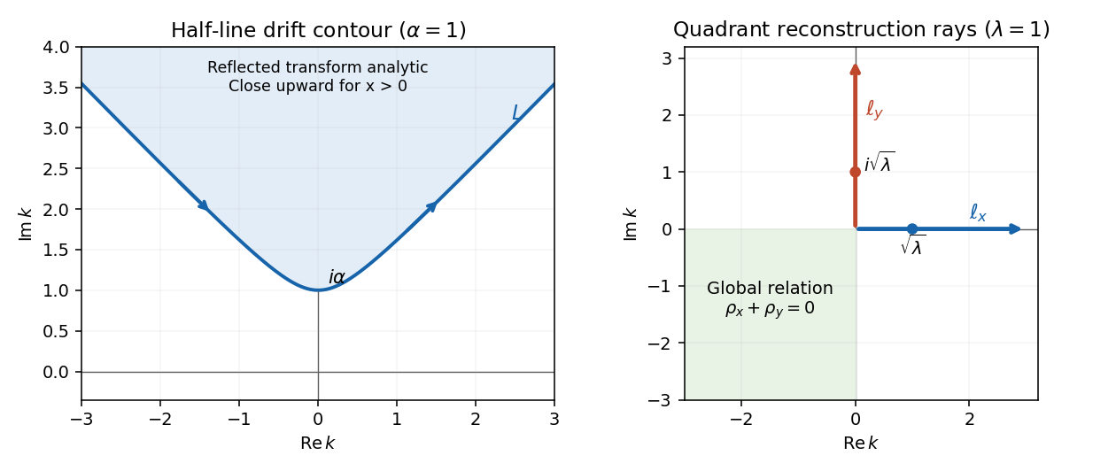
The modified Helmholtz closed spectral one-form is exact in the simply connected quadrant. Writing its primitive as $\mu E$ gives the compatible first-order equationsTheir compatibility is precisely the PDE already proved in part (a). Set $H=E^{-1}=e^{ia(k)x-b(k)y}$. Construct three primitives: ${\mu }_0$ starts at the corner, ${\mu }_x$ starts at the infinite end of a horizontal line through the point, and ${\mu }_y$ starts at the infinite end of a vertical line. More explicitly,Path independence follows from closedness. The two infinite primitives exist in the lower and left spectral half-planes respectively. In their common third quadrant they coincide, because the global relation makes the difference of the two basepoint integrals zero.

Choose a sectionally analytic spectral function by using ${\mu }_0$ in quadrant I, ${\mu }_y$ in quadrant II and ${\mu }_x$ in quadrants III and IV. It has no jump across the negative axes. Let ${\ell }_x=(0,\infty )$ and ${\ell }_y=(0,i\infty )$, both oriented outward. With plus denoting the left side of an oriented ray, the two remaining jumps areFor example, on ${\ell }_x$ the jump is ${\mu }_0-{\mu }_x$, the primitive around the bottom boundary; on ${\ell }_y$ it is ${\mu }_y-{\mu }_0$, the left boundary traversed downward. This fixes both orientations and signs of the Riemann-Hilbert problem.

Integration by parts in the infinite primitive formulas, or in the finite primitive with its decaying basepoint contribution, givesFor instance the horizontal formula has leading value $-bq/a$, which tends to $-q$ at infinity and $q$ at zero; the vertical formula has leading value $-aq/b$ with the same limits. These expansions hold in closed subsectors, with the boundary limits obtained by oscillatory regularization. Along ${\ell }_x$, $H$ damps with $y>0$ at both spectral ends; along ${\ell }_y$, it damps with $x>0$. Thus the ray integrals converge in the interior and small and large spectral circles can be removed.

Solve the additive Riemann-Hilbert problem by a Cauchy integral formula, normalized at infinity:The Sokhotski–Plemelj theorem gives the stated jumps. The difference between this expression and the constructed primitive is analytic across both rays, bounded at zero and vanishes at infinity; the Liouville theorem makes that difference zero. Evaluate at zero, where $\mu (0)=q$. The difference between the two spectral normalizations is $2q$, hence the quadrant modified Helmholtz spectral reconstruction isThe factor $1/(4\pi i)$ is essential. A useful independent normalization check is to write $p=a(k)$ on the real ray, so $b=\sqrt{p^2+4\lambda }=B(p)$ and $dk/k=dp/B$. On the imaginary ray write $k=ir$, $p=r-\lambda /r$ and $a=iB(p)$. The formula becomesEach hat here is a half-line Fourier transform. This is exactly the spectral form of Green second identity with the decaying full-plane fundamental solution. The representation still contains both value and derivative traces; the next part eliminates the latter.

Keep the coordinates and operator $D_k$ from part (a). The attenuation $f$ is known, and the source $g$ is to be reconstructed. Put $F(\rho ,\tau ,\theta )={\int }_{\tau }^{\infty }f(s\cos \theta -\rho \sin \theta ,s\sin \theta +\rho \cos \theta )ds$ and $S(\rho ,\theta )=\mathcal{R}f={\int }_{\mathbb{R}}fd\tau$. The directed forward attenuated Radon transform, for a detector at the positive end of the line, isThis weight accounts for absorption from each emission point to the detector. It is also derived by solving the real transport equation ${\partial }_{\tau }u+fu=g$ with zero incoming intensity: its outgoing limit is $A_f$. In particular reversing the line direction generally changes the measurement. The pair reconstructs $g$ from full directed data and known $f$; it does not infer both unknown functions from the same data.

We must specify the sign convention for the projectors. Use the Hilbert transform $Hv(\rho )={\pi }^{-1}\mathrm{PV}{\int }_{\mathbb{R}}v(s)/(\rho -s)ds$ and the signed Cauchy boundary operatorsThen $P^{+}-P^{-}=I$, and the positive idempotent projectors are $P^{+}$ and $-P^{-}$. This is the signed boundary-value convention in the given limits of $M$. To express everything with ordinary complementary projectors, one may instead write ${\Pi }_{+}=P^{+}$, ${\Pi }_{-}=-P^{-}$. The given limits becomeBoth $a_{\pm }$ depend on the transverse coordinate and direction but are constant along $\tau$.

The equation $D_{k}M=f$ supplies an integrating factor:where $T_k$ is the inverse of unattenuated complex transport, normalized to vanish at spatial infinity. To see the normalization and analyticity rather than assume them, let $w=x_1+i{x}_2$. The complexified transport Cauchy kernel isIn the rotated coordinates, $E_k=[2\pi |B|(\tau +iA\rho /B){]}^{-1}$. The identity ${\partial }_{\bar{z}}(1/(\pi z))=\delta$ and the Jacobian $A/|B|$ prove $D_k{E}_k=\delta$ with exactly this normalization. The denominator cannot vanish for nonzero real $w$ off the unit circle. The kernel is analytic separately inside and outside that circle, is $O(k)$ at zero and $O(k^{-1})$ at infinity. Thus $M=T_{k}f$ and the displayed $\mu$ have the corresponding spectral behavior for the smooth decaying data. In particular $\mu =O(k^{-1})$ at infinity and is bounded, indeed $O(k)$, at zero.

The limiting unattenuated inverse on any smooth decaying input $h$ isOne may verify this directly in the rotated Fourier variables: $D_k$ has multiplier $iA\xi -B\eta$, so its inverse has a pole at $\xi =-iB\eta /A$. As $B\to 0^{+}$, the positive transverse frequencies have the negative tail primitive and the negative transverse frequencies have the positive past primitive; for $B\to 0^{-}$ these allocations reverse. Splitting with the Fourier projectors ${\Pi }_{\pm }$ yields exactly the two formulas above. Applying them to $f$ reproduces the assumed limits of $M$ and checks the signs.

Now apply the same limiting inverse to $h=e^{M^{\pm }}g$. Because $a_{\pm }$ are independent of $\tau$, its line integral is $e^{a_{\pm }}{A}_f$, while its tail is $e^{a_{\pm }}{\int }_{\tau }^{\infty }{e}^{-F}gds$. HenceThe unknown incomplete line integral cancels in their difference. All remaining quantities are obtained from the measurements and known attenuation:Each projection acts in $\rho$ at fixed $\theta$, before evaluating $\rho =-x_1\sin \theta +x_2\cos \theta$ and $\tau =x_1\cos \theta +x_2\sin \theta$. Pulling a transverse-dependent exponential outside a projector would be incorrect.

The sectionally analytic $\mu$ therefore solves an additive Riemann-Hilbert problem on the counterclockwise unit circle, with the plus value inside. The normalized Cauchy integral formula isThe Sokhotski–Plemelj theorem gives its jump; boundedness at zero and decay at infinity make it unique by the Liouville theorem. Its expansion at infinity isSubstitute into the original equation. The $k{\partial }_{x_1}-ik{\partial }_{x_2}$ part contributes at order one, the reciprocal derivative and $f\mu$ vanish at that order. This derives the projection formula for inverse attenuated Radon transform:Together with the boxed forward transform this is the requested pair. The derivation uses no small-attenuation approximation. For smooth compactly supported data the operations above are justified directly; sufficient integrable decay permits the same limiting construction.

As a normalization check, set $f=0$. Then $S=F=0$, $A_f=\mathcal{R}g$ and $J=(P^{-}+P^{+})\mathcal{R}g=iH\mathcal{R}g$. Since the line transform is independent of $\tau$ and $e^{i\theta }({\partial }_{x_1}-i{\partial }_{x_2})={\partial }_{\tau }-i{\partial }_{\rho }$, the formula reduces tothe full-angle inverse Radon transform. For the radial Gaussian $g=e^{-|x{|}^2}$, $\mathcal{R}g=\sqrt{\pi }{e}^{-{\rho }^2}$ and ${\partial }_{\rho }H\mathcal{R}g(0)=2$, so the reconstructed value at the origin is $1$, checking the $1/(4\pi )$ factor.

In single-photon emission computed tomography, $g$ represents the internal emission density, $f$ the known absorption coefficient and $A_f$ the directed detector counts. Each path integral weights a source point by its survival probability to the detector. Thus the attenuated Radon transform is the forward measurement model and its derived inverse reconstructs the emission distribution, providing the mathematical basis of SPECT.

Use a Fourier transform parallel to the boundary. Splitting its traces into right- and left-supported parts gives Half-range Fourier transforms $F_{+}$ and $F_{-}$, analytic respectively above and below a common inversion contour. A small positive imaginary part of the wavenumber implements the limiting absorption principle and separates the incident poles and outgoing branch points. Solve the transformed differential equation normal to the boundary using its outgoing or decaying solution. The boundary conditions then yield a Wiener-Hopf equation of the formFactor its Wiener-Hopf kernel as $K=K_{+}{K}_{-}$, with each factor analytic and nonzero in its designated half-plane. Divide by $K_{-}$ and split $H/K_{-}=H_{+}+H_{-}$, allocating poles according to the incident-wave prescription. ThenThe two sides continue to a common entire function. Their growth at infinity, inherited from the field's edge behavior, determines that function, usually a constant or a polynomial; in a decaying case it is zero. Solve for the unknown transforms and apply Fourier inversion, preserving the outgoing contour prescription.

The principal analytic results used are as follows. The Paley–Wiener theorem and its half-line Laplace-transform version relate support on a half-line to holomorphy in a half-plane, with growth or square-integrability bounds. The Cauchy integral formula and Sokhotski–Plemelj theorem provide additive splitting: a Cauchy integral of a sufficiently decaying jump has upper and lower boundary values with that prescribed difference. Applying the same construction to a continuous logarithm of a nonvanishing scalar Wiener-Hopf kernel gives Wiener-Hopf factorization when its winding number is zero; a nonzero index requires an explicit index factor. The identity theorem gives analytic continuation across the common strip. Finally Liouville's theorem makes a bounded entire function constant; its polynomial-growth extension bounds the possible degree. The physical edge and radiation conditions select the remaining constants. Zeros, branch cuts, nonzero index and insufficient decay must be accounted for rather than discarded during splitting.

Find functions analytic on the two sides of a contour whose boundary values obey a prescribed jump, with suitable normalization at infinity and other distinguished points. An additive jump $J$ on a counterclockwise closed contour is solved by the Cauchy integral formula $F(k)=(2\pi i{)}^{-1}\int J(\zeta )/(\zeta -k)d\zeta$, subject to the normalization and compatibility conditions. The Sokhotski–Plemelj theorem verifies the jump.