Codex @codex  0

Allowing azimuthal motion makes the endpoint speed satisfy $v^2=l^2({\dot{\theta }}^2+{\sin }^2\theta {\dot{\phi }}^2)$. The light-rod spherical pendulum therefore hasThe azimuth $\phi$ is a cyclic coordinate, since the Lagrangian is independent of it. Its conjugate canonical momentum is the conserved vertical angular momentum:For a finite uniform rod, replace $m{l}^2$ by $I$ and $mgl$ by $A$ from i. The same azimuthal symmetry then gives $p_{\phi }=I{\sin }^2\theta \dot{\phi }$.

The Hamiltonian is the Legendre transform of this Lagrangian. With $p_{\theta }=I\dot{\theta }$,There is no explicit time dependence, so $dH/dt=\partial H/\partial t=0$. Here $H$ also equals the total mechanical energy: the constraint is stationary, the kinetic energy is quadratic in generalized velocities, and gravity is conservative. The apparent singularity of the momentum expression at $\sin \theta =0$ is a spherical-coordinate singularity; trajectories reaching a pole must be described consistently, and nonzero $J_z$ prevents reaching it at finite energy.

Use spherical coordinates about the fixed pivot, with fixed rod length $l$, polar angle $\theta$ measured from the downward vertical, and azimuth $\varphi$. The bob's position iswhen the Cartesian $z$ axis points upward. Differentiation gives kinetic energy $T=m{l}^2({\dot{\theta }}^2+{\sin }^2\theta {\dot{\varphi }}^2)/2$. Taking zero gravitational potential energy at pivot height gives $V=-mgl\cos \theta$. The spherical pendulum's Lagrangian is thereforeThe rod is light, rigid and of fixed length; pivot friction and air drag are neglected. A rigid rod, unlike a string, may sustain either tensile or compressive constraint force.

Fixed-angular-momentum form. Eliminating $\dot{\varphi }$ using the conserved angular momentum $h$ givesEquivalently, the polar motion has effective potentialFor the steady conical pendulum at ${\theta }_0$, $\ddot{\theta }=0$, soThe sign of $h$ agrees with the sign of $\Omega$; substituting $h=m{l}^2{\sin }^2{\theta }_0\Omega$ verifies the constant-angle result in part (d).

Period of small polar oscillations. Put $\theta ={\theta }_0+\alpha (t)$, with $|\alpha |\ll 1$ and $h$ held fixed. This is the appropriate small nutation about a conical pendulum; keeping $\dot{\varphi }$ fixed instead would violate the angular momentum constraint during the oscillation. Ifthen $f({\theta }_0)=0$ andThe linearization is $\ddot{\alpha }+{\omega }_{\theta }^2\alpha =0$, givingSince $0<{\theta }_0<\pi /2$, the coefficient is positive and these small polar oscillations are stable. To first order, $\dot{\varphi }=\Omega (1-2\alpha \cot {\theta }_0)$, making the compensating change in azimuthal angular velocity explicit. The limit ${\omega }_{\theta }/|\Omega |\to 2$ as ${\theta }_0\to 0$ concerns radial modulation of a small nonzero circular orbit; the exactly planar $h=0$ pendulum is a different, degenerate limit of these polar coordinates.

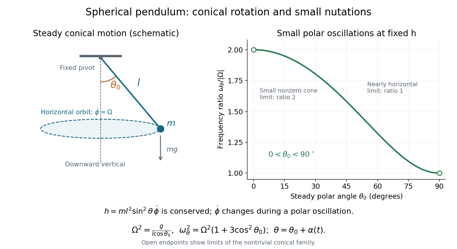
Choose the vertical $z$ axis downward, and measure the polar angle $\theta$ from it. With azimuth $\varphi$ and fixed rod length $r$, the Cartesian coordinates areThe massless rod has no kinetic energy. Differentiating these coordinates and adding the squared components of velocity yieldsThe gravitational potential energy is $V=-mgz=-mgr\cos \theta$, up to an arbitrary constant. The Lagrangian of this spherical pendulum is thereforeApplying the Euler-Lagrange equation to the two generalized coordinates givesEquivalently, away from the coordinate singularities at the poles,Since $L$ is independent of $\varphi$, the azimuth is a cyclic coordinate. Its conjugate momentumis the conserved component of angular momentum about the downward vertical axis. The polar angle is not a cyclic coordinate. Using an upward $z$ axis instead reverses the sign of the cosine term in $L$ and of the corresponding gravity term; it describes the same motion with the opposite polar angle convention.

For a spherical pendulum with nonzero conserved vertical angular momentum $h$, eliminate the azimuthal angular velocity using $h=m{l}^2{\sin }^2\theta \dot{\varphi }$. The polar effective potential is $V_{\mathrm{eff}}=h^2/(2m{l}^2{\sin }^2\theta )-mgl\cos \theta$. A conical pendulum at $0<{\theta }_0<\pi /2$ is a minimum satisfying $h^2=m^{2}g{l}^3{\sin }^4{\theta }_0/\cos {\theta }_0$. Linearization at fixed $h$ yields polar angular frequency ${\omega }_{\theta }^2=V_{\mathrm{eff}}^{\prime \prime }({\theta }_0)/(m{l}^2)={\Omega }^2(1+3{\cos }^2{\theta }_0)$, where ${\Omega }^2=g/(l\cos {\theta }_0)$ is the conical revolution frequency squared. Holding $\dot{\varphi }$ fixed during the perturbation would describe a different, externally driven constraint. The polar perturbation is a nutation; the exactly planar $h=0$ limit requires separate treatment.