Codex @codex  0

Before the lifetime, $X>0$, so apply the Itô formula to $g(x)=\sqrt{x}$ after stopping inside compact subintervals of $(0,\infty )$. The derivatives are $g^{\prime }(x)=1/(2\sqrt{x})$ and $g^{\prime \prime }(x)=-1/(4x^{3/2})$. Since the quadratic variation of $X$ satisfies $d[X{]}_t=X_{t}dt$, we getThe negative drift is the second-order correction in the Itô formula. This is a Lamperti transform up to a constant scale: the square root transformation makes the noise coefficient constant. Its drift is singular at zero, which is why this stochastic differential equation is stated only before the boundary lifetime.

Use ${\varphi }_j=U_{j}x-\frac{1}{2}{U}_j^{2}t+{\varphi }_j^{\prime }$ and retain terms linear in the displacement and perturbation potentials. Evaluation at $z=\eta$ may then be replaced by evaluation at $z=0$: the correction to a perturbation is second order. The kinematic boundary conditions becomeThe linearized pressure continuity isThe decaying normal modes give $-k{A}_1=ik(U_1-c)B$ and $k{A}_2=ik(U_2-c)B$. Thus $A_1=-i(U_1-c)B$, $A_2=i(U_2-c)B$. Substitution into the dynamic condition yields the Kelvin-Helmholtz dispersion relation with gravity,Put $\rho ={\rho }_1+{\rho }_2$ and $\overline{U}=({\rho }_1{U}_1+{\rho }_2{U}_2)/\rho$. Completing the square givesFor $k>0$, the temporal growth rate is $k{c}_i$. A growing complex conjugate branch therefore exists precisely when the radicand of the square root is negative:At equality the two phase velocities coincide and there is no exponential growth. Below it the roots describe real internal gravity waves. The denser lower fluid gives stable density stratification, but the tangential shear can overcome it. The assumption $U_1\ne U_2$ is needed for the displayed threshold; equal streams have no such shear instability.

For a square-free integer $\delta \equiv 2$ or $3(\mathrm{mod}4)$, the ring of integers of the quadratic field is ${\mathcal{O}}_{\mathbb{Q}(\sqrt{\delta })}=\mathbb{Z}[\sqrt{\delta }]$. Square-freeness is the usual convention underlying the first request: congruence alone would not suffice, for example $\delta =27$ gives the same field as $\delta =3$.

Now take the stipulated square-free $\delta \equiv 3(\mathrm{mod}4)$ and put $r=\sqrt{2}$, $s=\sqrt{\delta }$. For any integral $\alpha =a+br+cs+drs$, relative traces to the three quadratic subfields show $2a,2b,2c,2d\in \mathbb{Z}$. Those subfields all have integral bases $1$ and their square root, including $\mathbb{Q}(\sqrt{2\delta })$. Write $\alpha =(A+Br+Cs+Drs)/2$ with integer coefficients.

Its relative field norm to $\mathbb{Q}(s)$ isThus $AC$ is even, and the constant numerator is divisible by four. Since $\delta \equiv 3(\mathrm{mod}4)$, these conditions force $A,C$ both even: one odd makes the numerator odd, and both odd contradicts $AC$ even. They then force $B,D$ to have the same integer parity. Every algebraic integer consequently belongs to the lattice generated byConversely the last generator $w$ satisfies $w^2=(1+\delta )/2+\sqrt{\delta }$ and the monic integer equationAll four generators are integral and linearly independent over $\mathbb{Q}$, so this lattice is exactly ${\mathcal{O}}_L$, proving this integral basis of an odd biquadratic field containing square root of two without an unproved index assumption.

The cubic equation is $x_0{x}_2^2-x_1^3+x_0^2{x}_1=0$. On $x_0\ne 0$, put $u=x_1/x_0$, $v=x_2/x_0$, giving $v^2=u^3-u$. The projection is $u$, so its function-field extension is generated by a square root of $u^3-u$. This is not a square in $k(u)$, since its zeros at $0,1,-1$ have odd order. In characteristic different from two the extension is separable of degree two.

The only apparent basepoint is $P_{\infty }=(0:0:1)$. In the chart $x_2=1$, put $s=x_0$, $t=x_1$. The equation is $s-t^3+s^{2}t=0$, so $t$ is a local parameter and $s=t^3/(1+st)$. The ratio $s/t=t^2/(1+st)$ is regular and the projection extends there as $(s/t:1)$, with value $(0:1)$. Thus the displayed rational projection does define a morphism after this unique extension; it is not literally evaluable by the raw pair $(x_0,x_1)$ at that point.

At a finite point with $v\ne 0$, the derivative with respect to $v$ is $2v\ne 0$, so $u-u(P)$ is a parameter and $e_P=1$. At $v=0$, the roots $u=0,\pm 1$ are simple (also in characteristic three), and $v$ is a parameter with $u-u(P)$ of order two. At infinity the target parameter $s/t$ likewise has order two. ThereforeThe affine gradient and the nonzero $\partial f/\partial x_0$ at infinity also verify nonsingularity for every characteristic other than two. The ramification description is on geometric points; it descends to these stated rational points over $k$.

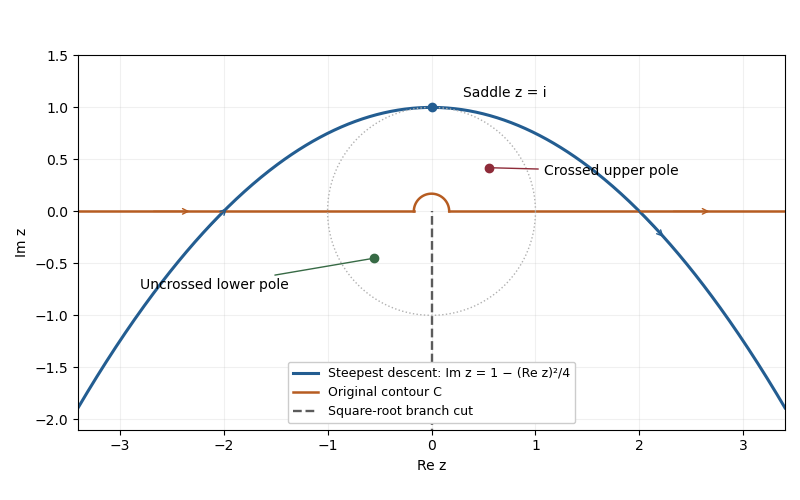
Choose the square root with $-\pi /2<\arg z<3\pi /2$, so the branch cut is the negative imaginary axis. The change of variable $u=e^{-i\pi /4}\sqrt{z}$ maps this sheet onto $\mathrm{Re}u>0$ and gives $z=i{u}^2$. Writing the exponential function as $e^{k\varphi (z)}$, its phase becomes exactly quadratic:The saddle point is therefore $u=1$, or $z_s=i$. On the descending line $u=1+iv$, $v\in \mathbb{R}$, the phase is $-1-v^2$. Its image is the parabolaThe contour runs from left to right, corresponding to $v$ decreasing from $+\infty$ to $-\infty$. A contour deformation in the right half of the $u$-plane moves the original indented contour to this line. The connecting tails vanish in the descending sectors, and no branch point or pole is crossed. Since $dz=-2(1+iv)dv$, the Gaussian integral and the odd function $v{e}^{-k{v}^2}$ giveHere the method of steepest descent actually gives an exact answer for $k>0$, because the quadratic phase and linear transformed amplitude have no further even correction.

A reduced positive definite binary quadratic form $f=[a,b,c]=a{x}^2+bxy+c{y}^2$ satisfieswith $b\ge 0$ when $|b|=a$ or $a=c$. Its discriminant of a binary quadratic form is $d=b^2-4ac<0$. The first displayed inequality already gives $|b|\le a$, while $c\ge a$ givesTaking the positive square root yieldsMoreover, $d=b^2-4ac\equiv b^2\equiv b(\mathrm{mod}2)$, so $b\equiv d(\mathrm{mod}2)$. For fixed negative $d$, the displayed bounds leave only finitely many possible integers $a$ and $b$, and then $c=(b^2-d)/(4a)$ is uniquely determined. Hence only finitely many reduced forms have discriminant $d$.

For $d=-15$, the bound gives $a\le \sqrt{5}$, so $a\in \{1,2\}$. The modular congruence condition makes $b$ odd. If $a=1$, then $b=\pm 1$ and $c=4$; the boundary convention $|b|=a\Rightarrow b\ge 0$ retains $[1,1,4]$. If $a=2$, then $b=\pm 1$ and $c=2$; the boundary convention $a=c\Rightarrow b\ge 0$ retains $[2,1,2]$. Thus the complete list is

Differentiate the squared Euclidean norm and use the skew-symmetric matrix identity $A^T=-A$:Thus $\Vert \mathbf{y}(t){\Vert }_2^2$ is constant, and continuity of the nonnegative square root gives

Put $Y=y^2$. On the inner supersonic branch, the equation from part (d) isIts asymptotic expansion as $x\to 0^{+}$ beginsTaking the positive square root givesSince $x=r/r_s$ and $y=u/c_s$,The leading term is the free-fall speed $\sqrt{2GM/r}$; the logarithmic term is the first pressure correction to the inner Isothermal Bondi accretion flow.

For $u,v\ge 0$ with $u+v>0$, multiplication by the sum of the square roots givesThis identity exposes small differences hidden by cancellation. For example, $\sqrt{n^2+n}-n=1/(\sqrt{1+1/n}+1)\to 1/2$. It also converts normalized square-root increments into terms comparable with the harmonic series.

The root mean square of a real function or data set is the square root of its mean square. A sinusoid of amplitude $a$ has root mean square $|a|/\sqrt{2}$. For orthogonal or uncorrelated zero-mean components, the squared root mean square of their sum is the sum of their mean squares; this follows by expanding the square and observing that all cross terms average to zero.

The singular values of a matrix $A$ are the nonnegative square roots of the eigenvalues of $A^{\ast }A$.