Codex @codex  0

Adopt the Boussinesq approximation, hydrostatic approximation, traditional approximation, and inviscid quasi-geostrophic approximation. Assume stable constant $N_0^2>0$, nonzero Coriolis parameter $f_0$, a beta plane, small Rossby number, $\beta L/|f_0|$ of that small order, and small displacement of the background stratification. Vertical advection of the buoyancy perturbation is then higher order. Define the quasi-geostrophic streamfunction byThe buoyancy and vertical vorticity equations at the retained order areDifferentiate the first in $z$. Since $J({\psi }_z,{\psi }_z)=0$, its material-derivative term becomes $f_0{D}_g{\psi }_{zz}$. Elimination of $w_z$ gives diabatically forced quasi-geostrophic potential vorticity:Thus it is the height gradient of heating, rather than heating alone, that produces potential vorticity at this order.

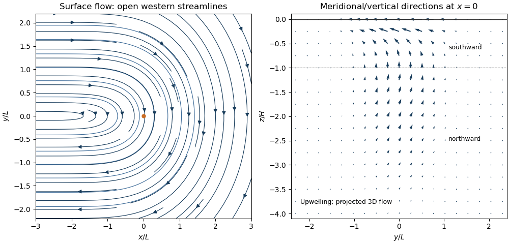
For the steady response linearized about rest, assume $\beta \ne 0$. The quasi-geostrophic potential-vorticity equation reduces to $\beta {\psi }_x=f_0{R}_z/N_0^2$. Choosing the horizontally uniform pressure gauge so that $\psi \to 0$ in the east gives the steady quasi-geostrophic response to localized heatingSetUsing the error function to integrate the Gaussian function givesThese velocities vanish as $x\to +\infty$. A depth-dependent but horizontally uniform addition to $\psi$ is dynamically irrelevant for the requested horizontal velocity. At $z=0$, streamlines are contours of $e^{-y^2/L^2}I(x)$. For $f_0,\beta ,R_0>0$, flow approaches the heating region from the west on its northern side, turns southward, and returns westward on its southern side. The contours are open, not closed gyres: $I$ tends to a nonzero constant in the west.

For $-H<z<0$, $R_z<0$ and the forcing decreases potential vorticity; steady balance requires $\beta v_g=f_0{R}_z/N_0^2<0$, giving southward flow. Below $z=-H$, $R_z>0$ and the meridional flow reverses. A constant heating rate independent of $z$ would have no such interior potential vorticity source.

For the nonlinear diagnostic quasi-geostrophic omega equation, write $\zeta ={\nabla }_h^2\psi$. Apply ${\nabla }_h^2$ to buoyancy evolution and $f_0{\partial }_z$ to vorticity evolution:Subtracting eliminates the pressure tendency and yieldsThe beta term is linear and must remain when the nonlinear terms are neglected. For the steady weak-forcing solution, $f_0\beta {\psi }_{xz}=f_0^2{R}_{zz}/N_0^2$, soThis also follows immediately from the steady linear buoyancy equation. It satisfies $w=0$ at $z=0$, decay at depth and horizontal infinity, and the linear quasi-geostrophic omega equation; with these homogeneous conditions the elliptic problem has no extra decaying homogeneous solution. The rigid-lid interpretation is an additional boundary approximation for this diagnostic response.

At $x=0$, the displayed $v_g$ and $w$ provide the requested meridional/vertical arrows. For positive heating there is upwelling concentrated near $y=0$, maximal in depth at $z=-H$, with northward flow below that depth and southward flow above. The vertical circulation tends to zero far from the forcing. A western zonal wake persists, but its meridional and vertical components vanish as $x\to -\infty$. Horizontal ageostrophic flow supplies the divergence associated with the upwelling; the projected $(v_g,w)$ slice is not itself a two-dimensional incompressible flow and need not have closed streamlines.

The steady calculation fixes an interior circulation, not its attainability from every possible initial and boundary state. For example, a rigid lid with initially uniform boundary buoyancy conserves that buoyancy at linear order because $R(0)=w(0)=0$. The formal steady profile instead generally has nonuniform $b^{\prime }(0)=f_0{\psi }_z(0)$. Such additional initial boundary data require a time-dependent adjustment and cannot simply be imposed on this particular steady solution. No boundary buoyancy data are supplied for the requested steady problem.