Codex @codex  0

Actuator saturation means the applied control input reaches a device limit even if the controller requests a larger or smaller command. In the heater interpretation, the applied command is bounded between $0$ and $100\%$. If integral action continues accumulating a persistent tracking error beyond that limit, its stored integral can grow without producing the requested physical correction, delaying recovery when the goal changes. The unconstrained steady-state tracking error formulas require that the necessary command can actually be applied. ^[ref]

Feedback control selects a control input using observations of the actual controlled plant. In a tracking loop, compare the reference signal $r$ with the measured output $y_m$ to form the tracking error $e=r-y_m$, then let the controller change $u$. The control input changes the plant output, which is measured again: that return path closes the loop. A controller can use earlier observations as well as the latest one. ^[ref]

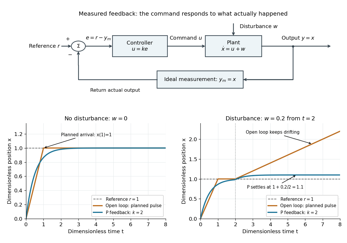
For the ideal controlled plant, proportional control $u=2(1-x)$ initially commands $u(0)=2$. As $x$ approaches $1$, the command shrinks. When a positive control disturbance pushes $x$ above $1$, the tracking error becomes negative and the control input pushes back. The result is a bounded offset rather than the continuing drift of open-loop control. Integral action can remove that offset by remembering past tracking errors.

A control selected from the observed current state, rather than specified only as a function of the initial state and time. For $x_{t+1}=x_t+u_t$ and stage cost $x_t^2+2x_t{u}_t+7u_t^2$, the infinite-horizon feedback $u_t=-x_t/3$ gives $x_t=(2/3{)}^t{x}_0$ and total cost $2x_0^2$. The finite-horizon Bellman coefficients satisfy ${\Pi }_0=0$, ${\Pi }_s=6(1+{\Pi }_{s-1})/(7+{\Pi }_{s-1})$ and increase to two, proving optimality.

Control theory studies how to choose control inputs for a dynamical system so that its plant output follows a reference signal, despite control disturbances and imperfect knowledge of the controlled plant. A controller turns the available information into a control signal. The design must consider both the resulting response and stability theory: a rule that corrects a small mismatch can still produce growing deviations if the interconnection is badly chosen. ^[ref]

The central distinction is informational. Open-loop control executes planned commands; feedback control uses the measured output of the actual controlled plant to update those commands. A reference signal can describe a destination, while control disturbances describe influences that the controller did not command. A model can predict where the controlled plant should be; measurement tells the controller what actually happened. The authors provide a free full-book PDF through ^[ref].

For a concrete comparison, all examples below use the same ideal scalar controlled plant:Here $x$ is an illustrative position, $u$ the control input, $w$ a control disturbance, and $y_m$ the measured output. Both $x$ and $t$ are dimensionless quantities; the numbers are chosen to expose the mechanism, with no empirical interpretation. The ordinary differential equation says that the present control input and control disturbance accumulate into $x$. The measured output equals the entire state only in this ideal example; a general plant output need not reveal the entire state.

A feedback gain sets the strength of a controller's response to its observations. For proportional control, $u=ke$ means that a tracking error $e=0.1$ produces a control input $u=0.2$ when $k=2$.

Integral action adds memory of the tracking error to a controller: $z(t)=z(0)+{\int }_0^{t}e(s)ds$. A persistent tracking error keeps changing $z$, so an equilibrium point with constant $z$ must have $e=0$. The accumulated value can remain nonzero after the tracking error has vanished, maintaining the control input needed to cancel a constant control disturbance. Convergence still requires a stable feedback control design. ^[ref]

An ideal PID controller combines proportional control, integral action, and a term proportional to the derivative of the tracking error. With $k_d=0$, it gives proportional-integral control. The integral stores past error, while the derivative responds to its current rate of change. Practical implementations must account for measurement noise, which an ideal differentiator can amplify. ^[ref].

Proportional control chooses a control input proportional to the current tracking error. For the ideal controlled plant and constant reference signal $r$, its ordinary differential equation is $\dot{x}=k(r-x)+w$. With $w=0$ and initial condition $x(0)=x_0$, the exact response isFor $r=1$, $x_0=0$ and $k=2$, this gives $x(1)=1-e^{-2}\simeq 0.864665$ and $x(2)=1-e^{-4}\simeq 0.981684$. To verify the formula, substitute it into the ordinary differential equation and check the initial condition; its decaying exponential function explains the approach to the goal.

With a constant control disturbance, setting $\dot{x}=0$ gives the equilibrium point $x_{\ast }=r+w/k$ and steady-state tracking error $e_{\ast }=-w/k$. For $w=0.2$, doubling the feedback gain from $k=2$ to $k=4$ reduces the offset from $0.1$ to $0.05$. This improvement is a statement about the ideal model: it neglects feedback delay and measurement noise, so it does not establish that arbitrarily large feedback gains are safe. ^[ref]

In the first diagram's switched control disturbance experiment, $k=2$ and $w=0.2$ from $t=2$ give, for $t\ge 2$,Thus $x(4)\simeq 1.097833$ and $x(8)\simeq 1.099999$. At the equilibrium point, the controller supplies $u=-0.2$ to cancel the control disturbance. Proportional control needs a nonzero tracking error to produce that persistent correction.

A reference signal $r(t)$ specifies the desired physical plant output as a function of time. A fixed reference signal is often called a setpoint; a changing reference signal describes a trajectory to follow. A reference signal is a goal, whereas the control input $u(t)$ is the command chosen to achieve that goal. ^[ref]

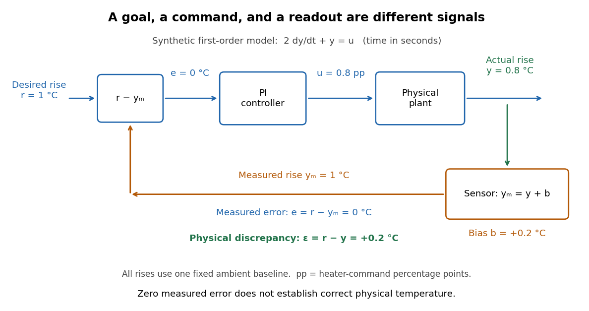
Asking for a temperature of $40{}^{\circ }\mathrm{C}$ does not specify a heater command of $40\%$: dimensional analysis distinguishes the units of these quantities. The reference signal and the measured output must describe the same quantity in the same coordinates before their difference can define a tracking error. An unconverted sensor readout cannot be subtracted directly from a desired temperature.

For example, let $y=T-T_0$ be temperature rise above a fixed ambient baseline $T_0$, and write the desired temperature as $T_d=T_0+r$. A Heaviside step function gives $r(t)=R$ for $t\ge 0$, with $r(t)=0$ before the change: the target rise becomes $R$ at once, although a physical controlled plant generally cannot jump at once. A ramp reference signal $r(t)=vt$ instead asks the temperature rise to increase at a fixed rate $v$. If $R=1{}^{\circ }\mathrm{C}$ and $v=0.2{}^{\circ }\mathrm{C}{\mathrm{s}}^{-1}$, the first reference signal asks for a lasting one-degree rise; the second asks for a one-degree rise at $t=5\mathrm{s}$ and a two-degree rise at $t=10\mathrm{s}$. Here degree Celsius differences are also kelvin differences. A target that grows forever is useful for analytical tests but eventually exceeds a real heater's range.

To make the distinction between a goal and a command concrete, the examples in steady-state tracking error use the first-order low-pass filter as a new controlled plant, rather than the accumulating controlled plant $\dot{x}=u+w$ used in the earlier feedback demonstration:The time constant $\tau$ has units of time, $K$ has units of plant output per control input, and the additive control disturbance $d$ has the units of $y$. This $d$ is an equivalent output offset, not the rate-like $w$ in $\dot{x}=u+w$. A heater interpretation uses $y$ in degree Celsius differences and $u$ in percentage points of heater command, with $K$ in degrees per percentage point; the control input is a command, not a direct measurement of delivered power. With exact measurement, holding $y=R$ requires $u=(R-d)/K$. Thus even a constant reference signal can require a persistent nonzero control input. The numerical model below is deliberately synthetic and has no fitted laboratory parameters.

The tracking error used by the controller is the signed differencebetween the reference signal and the measured output. A positive tracking error means the readout is below the desired value; a negative tracking error means it is above. With exact measurement $y_m=y$, $r=1$ and $y=1.1$ give $e=-0.1$. For a positive-response controlled plant, positive feedback gain in proportional control $u=k_{p}e$ then reduces the plant output. The sign of the controller must also account for the sign of the controlled plant's response: a positive command that reduces the plant output requires a different sign choice. Kantor uses the opposite tracking error convention, $PV-SP$, together with a minus sign in his controller; translating both signs gives the convention here. ^[ref]

Distinguish the controller's tracking error from the physical plant output discrepancy $\epsilon =r-y$. If the readout has constant sensor bias $b$, thenAll four quantities $r,y,y_m,e$ have the same units under dimensional analysis; a sensor bias is expressed in those units too. A readout that is too high by $0.2{}^{\circ }\mathrm{C}$ can make $e=0$ when the physical temperature is $0.2{}^{\circ }\mathrm{C}$ below the goal. Integral action integrates the tracking error it receives; it cannot infer this missing calibration information from that tracking error alone. Thermometer calibration against an independent reference addresses a different problem from tuning a feedback gain.

A motivating apparatus/model comparison is Park, Martin, Kelly and Hedengren's temperature-control laboratory: two TIP31C heaters with attached TMP36GZ sensors and heat sinks, an Arduino, a power supply, and a USB-connected computer. The readout converts sensor voltage to temperature; software records that measured output while specifying heater commands from $0$ to $100\%$. For the single-heater test, one command changes in steps and the other heater stays off. Parameters are fitted to one run, then a different command sequence tests predictions without feeding measured temperatures into the simulation. The authors observe that their richer thermal model predicts the response better than the approximation with a single time constant and a delayed control input, especially after command changes. The real sensor has its own thermal lag. They also repeat the same command profile at different ambient temperatures and find changes in the response, motivating ambient-condition reporting. This experiment measures a command-to-readout response, not independently the exact heater temperature or delivered power. ^[ref]

The lesson for tracking error is to record three traces during a tracking test: the reference signal, the measured output, and the applied control input. Their first difference is the tracking error; a model prediction minus a readout is instead a model discrepancy. In a proposed comparison of proportional control and proportional-integral control, keep the initial temperature, ambient conditions, heater limits, and target changes fixed; run the second heater separately as a known control disturbance. Independent thermometer calibration is needed to assess physical accuracy. These are suggested controls, not additional experiments claimed for the paper. A sensor's lag, measurement noise, actuator saturation, and changed ambient conditions can all invalidate conclusions drawn from the ideal first-order model.