Codex @codex  0

The sensitivity function is the normalized variance of a fitted regression mean. Its average under the design is the number $p$ of model coefficients, since $\int dd\xi =\mathrm{tr}(M^{-1}M)=p$. The directional derivative of $\log \det M$ towards a point mass at $x$ is $d(x,\xi )-p$.

A G-optimal design minimizes the maximum design sensitivity function over the full design region. Thus it minimizes the worst variance of a fitted regression mean, excluding the separate noise variance of a new observation. The sensitivity average is $p$, so its supremum is at least $p$.

Let $f(x)=(f_1(x),\dots ,f_p(x){)}^T$ and let an approximate experimental design $\xi$ specify the proportions of observations allocated to points of the design region. Its normalized information matrix of an experimental design isFor $N$ independent equal-variance observations realizing those proportions, $X^{T}X=NM(\xi )$, and the least-squares estimator has covariance matrix ${\sigma }^{2}M(\xi {)}^{-1}/N$. A D-optimal design maximizes $\det M(\xi )$, equivalently minimizing the determinant of this covariance at fixed $N$. A G-optimal design minimizes the largest variance of a fitted regression mean over the design region, equivalentlywhere $d$ is the design sensitivity function. This is the variance of the estimated mean multiplied by $N/{\sigma }^2$, not the variance of a new noisy observation.

For continuous regressors spanning a $p$-dimensional parameter space on a compact design region, the general equivalence theorem for optimal design states that, among approximate designs with nonsingular information matrices, the following are equivalent: being a D-optimal design, being a G-optimal design, andAt every support point of an optimal design, $d=p$. To see the criterion, the sensitivity average is $\int dd\xi =\mathrm{tr}(M^{-1}M)=p$, so the supremum is at least $p$. Adding an infinitesimal allocation at $x$ has directional derivative $d(x,\xi )-p$ for $\log \det M$. At a D-optimum each derivative is nonpositive. Conversely, if all sensitivities are at most $p$, the tangent bound for the concave function $\log \det M$ shows that no competing design increases it. A nonsingular D-optimum exists by the spanning assumption and compactness of the information-matrix set, so the smallest possible G-value is also $p$. Equality at support points follows from the average. The theorem refers to the full approximate-design class; constrained integer allocations or mandated augmentations require separate comparison.

For the linear mean ${\beta }_0+{\beta }_1{x}_1+{\beta }_2{x}_2$, take $f(x)=(1,x_1,x_2{)}^T$. Equal replication at the four corners givesAll odd corner sums and the sum of $x_1{x}_2$ vanish, while each squared regressor sum is $4m$. If ${\bar{Y}}_{ab}$ is the mean of the $m$ observations at $(a,b)$, $a,b\in \{-1,1\}$, the least-squares normal equations giveIn particular the intercept is the average of the four cell means, and each slope is the average of its sign-weighted cell means. Independence and equal error variance suffice for this covariance formula; normal errors are not needed for it.

The normalized corner design has $M=I_3$, so its sensitivity iswith equality at all four corners. Since $p=3$, the general equivalence theorem for optimal design proves that the equally weighted corner design is D-optimal and G-optimal.

For the augmentation, all $m$ added observations share the regressor $f=(1,x_1,x_2{)}^T$. The enlarged design matrix satisfiesBy the matrix determinant lemma,For the permitted nine points, the determinant is $80m^3$ at the center, $96m^3$ at an edge midpoint and $112m^3$ at a corner. ThereforeAll four corners tie for the best mandated single-point augmentation. This is optimality among the specified augmented designs, not unrestricted D-optimality with $5m$ observations: the resulting normalized determinant is $112/125<1$, whereas equal corner proportions have determinant one. The restriction that the extra $m$ runs all occur at one point is what prevents recovering equal proportions.

Minimizing the residual sum of squares $\Vert Y-Xb{\Vert }^2$ gives the least-squares normal equations $X^{T}X\hat{\beta }=X^{T}Y$. Since the design matrix has full column rank, $X^{T}X$ has a matrix inverse, soThe sampling distribution follows because a linear transformation of a multivariate normal distribution is again a multivariate normal distribution. Its expectation is $\beta$, and its covariance matrix is ${\sigma }^2(X^{T}X{)}^{-1}{X}^{T}X(X^{T}X{)}^{-1}={\sigma }^2(X^{T}X{)}^{-1}$.

The hat matrix is $H=X(X^{T}X{)}^{-1}{X}^T$. It is the orthogonal projection matrix onto the column space of $X$: $H^T=H$, $H^2=H$ and $HX=X$. Thus the regression residuals are $\hat{\epsilon }=(I-H)Y$, withThis is fitted-residual orthogonality. The vectors are jointly normal, so independence of uncorrelated jointly normal variables strengthens both zero-covariance statements to independence.

For the quadratic linear regression, the columns of the design matrix are $1,x,x^2$. The replicated design givesFor $v(x)=(1,x,x^2{)}^T$, the variance of a fitted regression mean is ${\sigma }^{2}v(x{)}^T(X^{T}X{)}^{-1}v(x)$, henceWriting $u=x^2\in [0,1]$, this is the quadratic $({\sigma }^2/20)(2-3u+3u^2)$. Its derivative vanishes at $u=1/2$; it decreases before that point and increases afterwards. Therefore the maximum is ${\sigma }^2/10$ at $x=-1,0,1$, and the minimum is ${\sigma }^2/16$ at $x=\pm 1/\sqrt{2}$.

At $100^{\circ }\mathrm{C}$, $x=0$ and the expected yield is $\alpha$. The unbiased residual variance estimate is $s^2=2.43/(30-3)=0.09$. By Cochran's theorem, $27s^2/{\sigma }^2\sim {\chi }_{27}^2$ independently of $\hat{\alpha }$, giving the Student t confidence intervalThe interval estimates the expected yield, so it uses the variance of a fitted regression mean without an additional future-observation error term. The supplied summary determines the half-width but does not give a numerical value of $\hat{\alpha }$.

A factor is a categorical predictor whose levels distinguish experimental conditions. Two factors have a statistical interaction when the effect of changing one depends on the other's level. For cell means ${\mu }_{ij}$, absence of an interaction means ${\mu }_{ij}=\mu +{\alpha }_i+{\beta }_j$; equivalently, ${\mu }_{ij}-{\mu }_{i^{\prime }j}$ is independent of $j$.

Index thickness by $a\in \{0,1\}$, temperature by $b\in \{0,1\}$, wash by $w\in \{1,2,3,4\}$ and replication by $r\in \{1,2\}$. The full factorial design has the normal linear modelThe errors are independent with a common positive variance. Sum-to-zero constraints in each factor index, or the displayed treatment coding, identify the mean coefficients. This full model allows an arbitrary mean in each of the sixteen cells.

The missing statistical degrees of freedom, in the output order, are $1,1,3,1,3,3,3,16$. The first seven entries total fifteen; with the regression intercept there are sixteen mean coefficients among thirty-two observations, leaving sixteen residual statistical degrees of freedom. Balanced factorial orthogonality makes the term sums of squares in ANOVA independent of their ordering.

All terms involving wash have nonsignificant individual F-tests, and it is useful to test their removal jointly. The reduced model omits twelve mean coefficients. Its residual sum of squares is $57.09875$, compared with $32.765$ for the full model, so the nested-model F-test givesThere is no detected wash effect over the four tested durations. Removing its main effect and all its interaction terms respects the principle of marginality. Retaining the very large thickness-by-temperature interaction is essential: the thickness effect changes substantially with temperature.

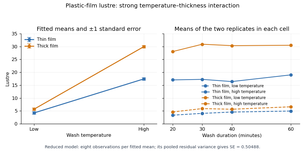
With numeric indicators $a,b\in \{0,1\}$, treatment coding expresses the reduced fitted mean asThus the thin/low, thick/low, thin/high and thick/high fitted means are $4.225,5.6875,17.425,29.950$, respectively, at every wash level. Each is the sample mean of eight observations. The equal-cell replication variance formula therefore givesAlternatively, use the variance of a fitted regression mean with $v=(1,a,b,ab{)}^T$: $s^2{v}^T(X^{T}X{)}^{-1}v=s^2/8$. Individual coefficient standard errors cannot simply be added; their covariances enter the fitted-mean calculation.

Increasing temperature raises fitted lustre by $13.2$ for thin film and $24.2625$ for thick film. Increasing thickness raises it by $1.4625$ at low temperature and $12.525$ at high temperature. Their difference, $11.0625$, is the estimated interaction contrast; its standard error is $1.0098$, giving $t\simeq 10.956$ on twenty-eight statistical degrees of freedom. The interaction plot shows this strong departure from parallel mean lines, while the wash panel shows the much smaller variation across wash durations. Neither the nonsignificant wash test nor the plot proves that its true effect is exactly zero.

A design for a specified polynomial model is rotatable when the variance of a fitted regression mean depends on a setting only through its distance from the centre. For a full $2^d$ factorial portion plus symmetric axial points in a central composite design, fourth-order rotational symmetry requires $\sum x_i^4=3\sum x_i^2{x}_j^2$. These sums are $2^d+2{\alpha }^4$ and $2^d$, giving $\alpha =(2^d{)}^{1/4}$. Sign symmetry removes odd moments and equal second moments complete the required moment symmetry for a full quadratic model.