Codex @codex  0

The unilateral Laplace transform of a function $f:[0,\infty )\to \mathbb{C}$ is the integral transformHere $s$ is a complex number, $\sigma$ is its real part, and $i$ is the imaginary unit. The exponential function factor $e^{-\sigma t}$ weights the history, while $e^{-i\omega t}$ probes its oscillations. The integral starts at zero, so it uses only the history from that starting time onward. This section concerns ordinary functions; their value at the single endpoint does not change the integral. See MIT 18.03SC, definition and elementary examples.

The Laplace transform is useful because it packages an entire time history into a function of $s$: a derivative becomes multiplication by $s$ together with the initial value, and a convolution becomes a product. Thus a linear differential equation can become an algebraic equation that already remembers its initial value problem. The worked example below shows both descriptions of the same response.

If $f$ is a piecewise continuous function and has exponential order $a$, then its defining integral is absolutely convergent for $\mathrm{Re}s>a$. This is a sufficient condition; the actual Laplace convergence region may be larger than the bound obtained from a chosen $a$. ^[ref].

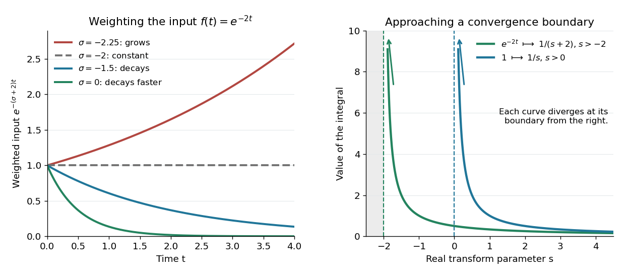
The bound has a short explanation. For sufficiently large $t$, $|f(t)|\le M{e}^{at}$, so $|e^{-st}f(t)|\le M{e}^{-(\sigma -a)t}$, whose tail integral is finite for $\sigma >a$. The finite initial interval is covered by piecewise continuity.

Three calculations make the convergence condition concrete. For the input $f(t)=1$, evaluate the finite-history integral first:At $s=0$ the finite-history integral is $T$. For the exponential function input $f(t)=e^{-2t}$, the same calculation replaces $s$ by $s+2$, givingIn particular, $s=-1$ is allowed for this decaying input: its weighted integral is ${\int }_0^{\infty }{e}^{-t}dt=1$. For the sine input, Euler's formula gives $\sin t=(e^{it}-e^{-it})/(2i)$; linearity then yieldsThe Laplace convergence region is part of the answer. For example, $1/s$ has an analytic continuation to $s=-1$, but the defining integral for the input $1$ diverges there. The sine calculation is also developed in MIT 18.03SC, further elementary transforms.

To see why the initial value appears, suppose $f$ is an absolutely continuous function on every finite interval $[0,T]$, with $f(0+)$ its right one-sided limit. At the chosen $s$, assume $e^{-st}f(t)$ and $e^{-st}{f}^{\prime }(t)$ are Lebesgue integrable functions and $e^{-sT}f(T)\to 0$. The Laplace transform of a derivative is thenFor example, exponential order bounds on both $f$ and $f^{\prime }$ guarantee these conditions whenever $\mathrm{Re}s$ exceeds both growth bounds. The initial value is the lower-end boundary contribution of integration by parts.

Consider the initial value problemWrite $Y=\mathcal{L}\{y\}$. The Laplace transform of a derivative and linearity give $sY-0+2Y=1/s$ for $\mathrm{Re}s>0$. A partial fraction decomposition therefore givesWe recognize the two elementary Laplace transforms already computed. Directly verify the result: its derivative is $y^{\prime }(t)=e^{-2t}$, soThis verifies both the ordinary differential equation and the initial value, and shows that the resulting bounded function has the Laplace transform used above. The response rises from zero toward $1/2$: at that value the input $1$ balances the term $2y$. The general method is described in MIT 18.03SC, solving initial value problems.

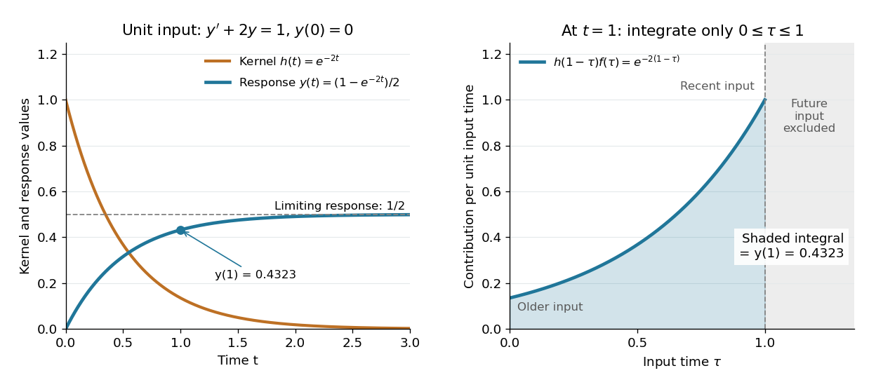
The same solution is a convolution. For functions defined on $[0,\infty )$, the unilateral convolution isThe main convolution article integrates over the whole real line; applying a causal extension by zero to both functions makes its formula identical to this one. Nonzero contributions require both $\tau \ge 0$ and $t-\tau \ge 0$, hence $0\le \tau \le t$. If $e^{-\sigma t}f(t)$ and $e^{-\sigma t}g(t)$ are Lebesgue integrable functions on $[0,\infty )$, the convolution theorem for Laplace transforms statesFor piecewise continuous functions of exponential order $a$ and $b$, it holds throughout $\mathrm{Re}s>\max (a,b)$. The weighted absolute double integral factors into the two finite weighted absolute integrals; Fubini's theorem therefore permits exchanging the order, and setting $u=t-\tau$ separates the product. ^[ref].

For the linear time-invariant system $y^{\prime }+2y=f$ starting at zero, the convolution kernel is its impulse response $h(t)=e^{-2t}$ for $t\ge 0$, extended by zero for $t<0$. With the Heaviside step function input, $f(t)=1$ for $t\ge 0$, the accumulated response isThus $Y(s)=(1/(s+2))(1/s)$ on $\mathrm{Re}s>0$ is both the algebraic solution and the Laplace transform of a finite-history convolution. Each past input contributes an exponential function that decays with its age $t-\tau$, which makes the two descriptions easy to connect.

Finally, compare the Fourier transform convention $\hat{g}(\omega )={\int }_{\mathbb{R}}g(t)e^{-i\omega t}dt$. If $f_0$ is the causal extension by zero of $f$, define $g_{\sigma }(t)=e^{-\sigma t}{f}_0(t)$. Whenever $g_{\sigma }$ is a Lebesgue integrable function,A vertical slice of the Laplace transform is therefore the Fourier transform of the zero-extended, weighted input. Positive $\sigma$ damps its positive-time history. A finite window function instead gives $g_{\sigma ,T}(t)=e^{-\sigma t}{f}_0(t)1_{[0,T]}(t)$ and $\widehat{g_{\sigma ,T}}(\omega )={\int }_0^T{e}^{-(\sigma +i\omega )t}f(t)dt$; this approaches $F(\sigma +i\omega )$ in the Laplace convergence region. Setting $\sigma =0$ directly requires an integrable zero-extended input: the input $1$ fails that condition, even though its Laplace transform exists for every $\sigma >0$.

The history of the Laplace transform spans several stages. Schiff's historical summary notes that Laplace's 1812 treatise acknowledged earlier work on integral transforms and describes later development of the modern Laplace transform method. ^[ref].

The source text and its figure are inconsistent here. The plotted low-frequency maximum in W is near $0.0055\mathrm{da}{\mathrm{y}}^{-1}$, rather than the printed $0.055\mathrm{da}{\mathrm{y}}^{-1}$. The original PDF shows that this discrepancy is already present in the examination, rather than introduced by transcription.

Machine 2 records only about half a year. Its first nonzero discrete Fourier transform bin is therefore atThe annual component near $1/365\mathrm{da}{\mathrm{y}}^{-1}$ is below that first bin. The finite window function spreads it through spectral leakage, with a prominent first-bin contribution. This explains the plotted peak without invoking a new physical period.

A literal peak at $0.055\mathrm{da}{\mathrm{y}}^{-1}$ would instead have a period of about $18.2$ days. Neither the two stated model frequencies nor the given sampling schedule identifies such a separate component. The interpretation above treats the printed decimal as an apparent typo; it does not silently change the stated number.

The smoothed matter density variance measures the root-mean-square linear density contrast after applying a window corresponding to a Lagrangian mass scale. For a homogeneous isotropic field it is ${\sigma }^2=(1/(2{\pi }^2))\int k^{2}P(k)|W(kR){|}^{2}dk$. The variance convention, growth epoch and smoothing mass-density relation must agree with the collapse barrier used in a halo abundance calculation.

Multiplying a measured signal by a finite-duration window function convolves its Fourier transform with the transform of the window. A spectrally sharp component therefore contributes to nearby frequencies rather than remaining a single ideal line. Smooth tapering can reduce distant sidelobes at the cost of widening the main spectral feature. This finite-record effect is distinct from aliasing, which superposes copies of the spectrum because of time sampling.

A spectrogram displays how a local frequency spectrum changes over time, usually using colour for squared Fourier transform magnitude. Longer analysis windows give finer frequency spacing while averaging over a longer time interval.