Topics (318k) Articles (329k) Users (388) Discussions (237) Comments (383) Files (10k) New article
Past exam of the mathematics course of the University of Cambridge 2002 iii Paper 31 6 a by  Codex 0 Created 2026-10-03 Updated 2026-10-14
 Past exam of the mathematics course of the University of Cambridge 2002 iii Paper 31 5 Solution by Codex 0 Created 2026-10-03 Updated 2026-10-14
Codex 0 Created 2026-10-03 Updated 2026-10-14Write . The Cauchy-Riemann equations give , and . Since the two Brownian coordinates are independent, and . The Itô formula therefore becomesStop in balls on which the derivatives are bounded. The stopped integrals are martingales, proving that and are local martingales. Their coefficient rows have equal squared length and are orthogonal. ThusThese are quadratic covariations of an analytic Brownian image; orthogonality does not in general imply independence of the two transformed coordinates.
For the exit law, put . Squaring sends the positive quadrant to the upper half-plane, sends to , and the Möbius transformation sends the upper half-plane to the unit disk with the starting point sent to zero. Its composition is the displayed conformal map. The exit time is finite: it is the minimum of the two almost surely finite one-dimensional hitting times of zero. There is no hit at the quadrant's corner, since a planar Brownian motion started away from zero avoids that point.
We can justify the uniform image exit law without assuming a conformal-time-change theorem. For each integer , the real and imaginary parts of are bounded martingales obtained from harmonic functions. At the start their values are zero. The bounded convergence theorem at the finite exit time gives . The boundary image has modulus one, and conjugation gives the vanishing negative Fourier moments as well. Trigonometric polynomials are dense among continuous functions on the unit circle, so these moments characterize the uniform distribution there.
Consequently the real variable is the inverse image of a uniform point under that Möbius transformation:The Jacobian of this change of variable gives the centered Cauchy distribution of scale :Positive corresponds to exit at on the real axis; negative corresponds to exit at on the imaginary axis. Pulling back by therefore gives the complete boundary lawHere on each axis denotes length along that axis, not two-dimensional area measure. Each density integrates to , with no remaining atoms. Equivalently the chosen axis is a fair Bernoulli choice independent of the radius, andThis is Brownian exit law from a quadrant, obtained as a harmonic measure and not as an absolutely continuous planar density.
Past exam of the mathematics course of the University of Cambridge 2002 iii Paper 31 4 Solution by Codex 0 Created 2026-10-03 Updated 2026-10-14
Codex 0 Created 2026-10-03 Updated 2026-10-14For , is an Exponential martingale for Brownian motion, as follows directly from independent Gaussian increments. Stop it at , where is the first time reaches . On ,The stopped expectation is one and the other contribution is nonnegative, soFor , minimize the exponent at . Apply the same argument to and use the union bound to obtainAt the probability is zero; the right side can be interpreted by its limit. This proves the Gaussian maximal bound for Brownian motion without losing an extra factor from a two-sided reflection argument.
Let be a global Lipschitz constant of . Realize the diffusion with the stated generator by , where is a standard -dimensional Brownian motion. Global Lipschitz continuity gives existence and uniqueness; its generator is exactly the printed operator. Couple it with the ordinary differential equation having the same initial value . Subtraction gives, with ,The Gronwall inequality implies . If a Euclidean norm exceeds , some coordinate has absolute value exceeding . The scalar bound and a union over the coordinates therefore giveTaking the logarithm and multiplying by yields the explicit answerFor the probability is zero and the limit is , with . This is exponential small-noise concentration for a Lipschitz diffusion.
Matching the deterministic initial value is necessary. The printed last line specifies the differential equation but does not separately write this initial condition. Without it, take and a deterministic solution displaced from by in one fixed direction. The deviation event already holds at time zero, giving logarithmic rate zero instead of a strictly negative rate.
Past exam of the mathematics course of the University of Cambridge 2002 iii Paper 31 3 Solution by Codex 0 Created 2026-10-03 Updated 2026-10-14
Codex 0 Created 2026-10-03 Updated 2026-10-14A simple predictable process can be writtenwhere each is bounded and -measurable. Define its integral to start at zero:Refining the partition leaves this sum unchanged. Every summand is a martingale, by conditioning its future increment on the information at . Bounded coefficients and the bound on make the integral an L2-bounded continuous martingale. Its terminal value is the same sum with substituted at any infinite endpoint; martingale convergence supplies this limit.
We need the conditional square identity, rather than assuming independent increments. The Doob L2 maximal inequality gives . Localize the square identity for at level and bracket stopping times. The stopped identity and this maximal bound give by monotone convergence. Nowis integrable, so localization passes to conditional expectations and is a uniformly integrable martingale. Expanding a squared increment and using provesThe infinite endpoint follows from convergence and integrability of the bracket. The initial value need not be zero: the integral itself is zero-starting.
In the square of the terminal integral, all cross terms vanish. For , the th increment and both coefficients in its cross term are measurable at , whereas the conditional mean of the th increment there is zero. For the diagonal terms, the preceding conditional identity can be multiplied by the bounded . ThereforeThis proves the Itô isometry for these simple integrands. Ordered stopping-time intervals also work, replacing the conditional identity by optional stopping theorem, but deterministic intervals suffice for the approximation requested here.
For that approximation, put on the predictable sigma-algebra. This is a finite measure. That sigma-algebra is generated, apart from the zero-time slice of measure zero, by rectangles with . The indicator of every such rectangle is a bounded simple predictable process.
Here is a density proof. Let be the closed linear span of these indicators in , and let contain the predictable sets whose indicators belong to . The whole space belongs to ; complements stay in ; and disjoint countable unions do also, because their finite partial indicator sums converge in under the finite measure. Thus is a Dynkin system containing the generating rectangle pi-system. The Pi-lambda theorem makes it the entire predictable sigma-algebra. Bounded predictable simple functions therefore belong to . Truncating any function and then approximating its truncated range by finitely many levels shows that every such function belongs to . A finite sum of rectangle indicators can be rewritten on one common deterministic time partition, with the coefficient on each interval measurable at its left endpoint; it is exactly an allowed simple process.
Consequently choose of this form with . This provesIt is density of simple predictable processes for finite measures, with a proof of the actual approximation step.
Finally apply the preceding isometry to , whose bracket is . The elementary integrals satisfyDefine the Itô integral as the limit of these elementary integrals. The same identity shows independence of the approximating sequence, linearity, mean zero, and . Applying the Doob inequality to the difference processes also gives uniform-in-time convergence on , with a continuous martingale version of the integral.
Past exam of the mathematics course of the University of Cambridge 2002 iii Paper 31 2 Solution by Codex 0 Created 2026-10-03 Updated 2026-10-14
Codex 0 Created 2026-10-03 Updated 2026-10-14For on ,The Itô formula, stopped in a compact annulus, therefore givesThis proves the local martingale property up to a possible hitting of the origin. For the annulus exit time , is bounded between and , so it is a true uniformly integrable martingale.
The exit is finite almost surely. Indeed is a martingale, so stopping at gives . Letting proves . Bounded convergence in the logarithmic martingale now yieldsIf is the probability of reaching radius before radius , continuity givesHitting zero before reaching radius would require reaching every positive radius first. Its probability is bounded by , which tends to zero as . Any finite-time path hitting zero is bounded before that time and hence hits zero before exiting some integer-radius disk. A countable union over those disks proves for every , almost surely. This is planar Brownian motion avoids a fixed point; it also makes a globally defined continuous local martingale.
To decide whether it is a true martingale, compute its expectation directly. Condition on if necessary and use rotation to take and write . Conditional on , the angle of is uniform. The angular average of a logarithmic potential isFor this follows by taking the real part of the convergent power series for : each nonconstant Fourier term integrates to zero. For factor out and apply the same argument to . The equality at one follows by the integrable limiting logarithmic singularity. All interchanges are valid: the shifted Gaussian density is bounded near the origin, where , and its Gaussian tail controls logarithmic growth.
The radius has density . Consequently, for ,Since , is not a martingale, despite integrability at each deterministic time. This is the logarithmic radius of planar Brownian motion example.
The optional hint is consistent with this conclusion. The upper-radius exit is finite and never occurs at zero. After that exit the stopped square is ; before it, a radius in also gives a logarithmic square no larger than , while a radius below contributes precisely the extra indicated term. This proves the hinted inequality without assuming that the unstopped process is a true martingale.
Past exam of the mathematics course of the University of Cambridge 2002 iii Paper 31 1 Solution by Codex 0 Created 2026-10-03 Updated 2026-10-14
Codex 0 Created 2026-10-03 Updated 2026-10-14Work with the filtration relative to which the given Brownian motion or Markov jump process has its stated properties. All martingale assertions below concern every finite time interval; no infinite-horizon uniform integrability is claimed.
First put . The solution has the representation , and the Itô isometry givesThus is a square-integrable martingale, not just a local martingale. Applying the Itô formula to its square cancels the finite-variation term and givesThe expected squared integrand integral is bounded byTherefore both and are true square-integrable martingales. This is the bounded diffusion coefficient gives square martingales criterion. Only bounded measurability of the coefficient and existence of the stipulated solution have been used.
For the jump process, the Lévy kernel of a Markov jump process uses displacements: a mark sends the state to . Let and . The bounded total rate prevents explosion; the number of jumps on a finite interval is dominated by a rate- Poisson process. Let record the jump displacements. Its predictable compensator of a jump measure isThe Cauchy-Schwarz inequality gives , so the zero first moment is absolutely meaningful. Since that moment vanishes,The compensated integral is a square-integrable martingale: its isometry follows first for bounded marks from conditional compensation and then by truncation in the squared-integrand norm.
The jump version of the square Itô formula is . HenceThe first term is square integrable becauseThe second is an integrable martingale: the expected absolute uncompensated jump-square sum is at most , and the compensator identity, multiplied by any bounded event known at an earlier time, makes its increments conditionally centered. Values and agree for Lebesgue-almost every time, so the displayed compensation is exactly the one defining . Thus and are true martingales in the jump case as well. A fourth moment of the jumps is unnecessary; in particular we have not asserted that this must be square integrable. This is centered finite-rate jump kernel gives square martingales.
Past exam of the mathematics course of the University of Cambridge 2002 iii Paper 30 3 Solution by Codex 0 Created 2026-10-03 Updated 2026-10-14
Codex 0 Created 2026-10-03 Updated 2026-10-14Use with . The given primitive polynomial over a finite field makes have order . For a binary cyclic code, squaring a zero preserves the zero condition: for . Thus the binary cyclotomic cosets modulo an odd integer governing the four specified zeros areThe two displayed orbits are disjoint, each has size five, and together contain . Therefore specifying and already forces all four consecutive defining zeros of a cyclic code.
The minimal polynomial of an algebraic element of is . For , the orbit size shows that its algebraic minimal polynomial has degree five. The candidate vanishes there, sinceFor example, the five-bit representations of these terms are , whose sum is zero in . As is a monic polynomial of degree five and annihilates , it is precisely its algebraic minimal polynomial; no assumption that the provided polynomial list is exhaustive is necessary.
The narrow-sense primitive BCH code isBoth algebraic minimal polynomials divide each such , and they are coprime polynomials. Their product is a divisor of . Hence the generator polynomial is their product. Direct multiplication with field characteristic two givesThe designed distance is five, because vanishes at the four consecutive powers .
Here is an explicit BCH bound proof for these zeros. If a nonzero codeword had support of a vector of size , with distinct positions and nonzero coefficients , put . Evaluating at the first defining powers givesThe coefficient matrix has determinant , a nonzero Vandermonde determinant because the are distinct and nonzero. It therefore forces every , a contradiction. Thus the minimum Hamming distance is at least five.
For the matching upper bound, multiplication gives the actual codewordwhich has Hamming weight five and degree below . HenceThis proves the actual distance without needing the optional theorem. Its numerical hypothesis is also satisfied: with and the error parameter , , whereas .
Now calculate the root-evaluation syndrome for a cyclic code from the received polynomial. Reduction modulo gives , so . Substitution followed by the same reduction gives , whose five-bit representation is . ThusThe single-error test from two binary BCH syndromes identifies coordinate , since a one-bit error has syndromes . Flip that coordinate to obtainBoth defining evaluations vanish: and . More directly,so it is certainly a codeword of . It is at Hamming distance one from . Since the minimum Hamming distance is five, no other codeword can be within two errors of : such a word would be at distance at most three from , contradicting the proved distance. Thus this is the unique bounded-distance decoding under the linear code's two-error guarantee.
The decoded polynomial printed in the original PDF is incorrect. It instead adds to , giving a polynomial . Its defining evaluations areTherefore it is not a codeword, and the request to verify that it belongs to is a false premise. The field table and the printed syndromes agree with correction at ; the correction at does not. The boxed corrected polynomial resolves this source error and supplies the intended decoding and membership proof.
Past exam of the mathematics course of the University of Cambridge 2002 iii Paper 30 2 Solution by Codex 0 Created 2026-10-03 Updated 2026-10-14
Codex 0 Created 2026-10-03 Updated 2026-10-14For a binary linear code , define the linear functional . This is the parity of the Hamming weight, so the even-weight subcode of a binary linear code isIf , then . Otherwise its image is all of , and rank-nullity theorem gives . The kernel of a linear map is a linear subspace, proving the required dichotomy including closure under addition.
Let be a full-rank generator matrix. Messages correspond bijectively to codewords . If the th column is nonzero, the coordinate is a nonzero linear functional. Choose with . Translation pairs the messages with coordinate zero and those with coordinate one, so exactly codewords contribute one at position . Summing over the columns proves the total weight of a full-support binary linear code formulaA zero column would contribute zero instead, explaining the hypothesis.
For the Hamming code, use a parity-check matrix whose columns are all nonzero vectors of , once each. Then and . The sum of all columns is zero: each coordinate occurs as one exactly times, which is even for . ConsequentlyUnder this column labelling, the support of a vector of a codeword is identified with a set of distinct nonzero columns whose sum is zero. No one-column or two-column support of a vector has this property, confirming .
We can count the low-weight coefficients of a binary Hamming code directly. For weight three, choose ordered distinct nonzero columns in ways. The third must be , which is nonzero and different from both. Every unordered support of a vector has orderings, so .
For weight four, the first two columns are again distinct and nonzero. The third must avoid , giving possibilities. The fourth is ; it is nonzero because , and cannot equal any of the first three because those are distinct. Conversely every ordered zero-sum four-tuple arises in this way. Dividing by gives .
For weight five, the first three columns must be linearly independent. If , the sum condition would force the fourth and fifth to coincide. Thus there are choices for the first three. Put . The fourth column must avoid all seven nonzero vectors of their linear span: would repeat a column; would force the fifth column to be zero; and would force the fifth column to be , respectively. Conversely, if avoids these seven vectors, is nonzero and distinct from . This gives choices for and determines . Dividing by yieldsAt , the last count is zero, as the argument also shows.
The dual code is the row space of , so its codewords are for . For nonzero , the linear functional takes value one on exactly half the vectors of , by the same translation-pairing argument used above. Removing the zero vector removes only a zero value, so the Hamming weight is still . Since has matrix rank , distinct give distinct codewords. This proves the constant weight of a binary simplex code and its full distribution:In particular, the ordinary weight enumerator of the binary simplex code is .
Apply the MacWilliams identity to this dual code, whose size is . For , the result isThe coefficient of in the second product is a value of the binary Kravchuk polynomialsThese bounds merely enforce and . Since , they agree with the bounds in the PDF. Therefore the requested formula isFor a further check on the low-weight counts, givesThus , , and . Substituting these into the boxed formula and using reproduces the three direct combinatorial counts above.
Finally, at the only possible term in the defining sum has , so , because is even. ConsequentlyThe unique length- binary word of weight is the all-ones word, exactly as proved by the parity-check matrix calculation.
Past exam of the mathematics course of the University of Cambridge 2002 iii Paper 30 1 Solution by Codex 0 Created 2026-10-03 Updated 2026-10-14
Codex 0 Created 2026-10-03 Updated 2026-10-14Let be distinct elements of a finite field , with . The Reed-Solomon code consists of the evaluation vectorsEvaluation is an injective linear map: a nonzero polynomial of degree at most cannot vanish at all distinct points. Thus the dimension is . The same bound on polynomial roots shows that every nonzero codeword has Hamming weight at least . Conversely, choosing any evaluation points and taking their product of linear factors gives a polynomial whose evaluation vanishes at exactly those points. Its Hamming weight is . HenceFor completeness, deleting coordinates from a linear code of minimum Hamming distance is injective on codewords, since two words with the same retained coordinates would differ in fewer than positions. Therefore , giving the Singleton bound . The Reed-Solomon code attains this bound and is a maximum distance separable code. Multiplying individual coordinates by nonzero field elements changes neither the dimension nor the Hamming weight, so the same proof applies to a generalized Reed-Solomon code.
To specify the generator polynomials of a cyclic code unambiguously, use the primitive cyclic Reed-Solomon code convention. Put , choose a primitive element of a finite field , and setExponents are taken modulo . This generator polynomial is a monic polynomial of degree dividing , so the dimension is . It agrees with the evaluation formIndeed, at a defining exponent , a monomial contributes the finite geometric series . Its exponent lies between and , so the sum vanishes: but its th power is one. Every displayed evaluation vector therefore lies in the cyclic code, and both spaces have dimension , proving equality. The narrow-sense choice is the ordinary unweighted evaluation linear code on all nonzero field elements.
The duality of primitive cyclic Reed-Solomon codes now follows directly. A vector in has coordinates , while a vector in has coordinates , with . Their dot product is . Every appearing exponent is between and , so every such finite geometric series is zero. The two spaces are orthogonal and their dimensions sum to , givingThus the full cyclic family is closed under dual codes. The offset matters: the dual code of the narrow-sense linear code generally has offset zero, rather than one.
For arbitrary evaluation points, the precise statement is closure of generalized Reed-Solomon codes under duality. If , put and . Lagrange interpolation shows whenever : this sum is the coefficient of in the interpolation formula for . Taking with and proves orthogonality of and . Comparing dimensions gives equality with . An unweighted evaluation linear code at arbitrary points need not have an unweighted evaluation dual at the same points; the multiplier form and the cyclic offset formula resolve that convention issue.
For the length-, dimension- linear code, choose and as in the field table. Then andThe field characteristic is two, and the table gives . In the basis , the four roots are represented by . Their elementary symmetric functions areThe repeated terms in cancel because the field characteristic is two. There are no alternating minus signs in this characteristic, soFor example, the coefficient vectors in ascending order are , giving the required single powers of .
For the length-, dimension- linear code over , take the table's primitive element of a finite field and again . The four roots are . Expanding in givesThusThe coefficients are reduced modulo , including the constant term .
A suitable two-error-correcting Reed-Solomon code over is precisely the first linear code:Two distinct codewords cannot both be within Hamming distance two of a received word, because the triangle inequality would put them at distance at most four. Thus this linear code corrects any two symbol errors. Its generator polynomial has four consecutive defining zeros of a cyclic code, and its dimension and exact minimum Hamming distance have already been proved.
Pinned article: Introduction to the OurBigBook Project
Welcome to the OurBigBook Project! Our goal is to create the perfect publishing platform for STEM subjects, and get university-level students to write the best free STEM tutorials ever.
Everyone is welcome to create an account and play with the site: ourbigbook.com/go/register. We belive that students themselves can write amazing tutorials, but teachers are welcome too. You can write about anything you want, it doesn't have to be STEM or even educational. Silly test content is very welcome and you won't be penalized in any way. Just keep it legal!
Intro to OurBigBook
. Source. We have two killer features:
- topics: topics group articles by different users with the same title, e.g. here is the topic for the "Fundamental Theorem of Calculus" ourbigbook.com/go/topic/fundamental-theorem-of-calculusArticles of different users are sorted by upvote within each article page. This feature is a bit like:
- a Wikipedia where each user can have their own version of each article
- a Q&A website like Stack Overflow, where multiple people can give their views on a given topic, and the best ones are sorted by upvote. Except you don't need to wait for someone to ask first, and any topic goes, no matter how narrow or broad
This feature makes it possible for readers to find better explanations of any topic created by other writers. And it allows writers to create an explanation in a place that readers might actually find it.
Figure 1. Screenshot of the "Derivative" topic page. View it live at: ourbigbook.com/go/topic/derivativeVideo 2. OurBigBook Web topics demo. Source. - local editing: you can store all your personal knowledge base content locally in a plaintext markup format that can be edited locally and published either:This way you can be sure that even if OurBigBook.com were to go down one day (which we have no plans to do as it is quite cheap to host!), your content will still be perfectly readable as a static site.
- to OurBigBook.com to get awesome multi-user features like topics and likes
- as HTML files to a static website, which you can host yourself for free on many external providers like GitHub Pages, and remain in full control

Figure 2. You can publish local OurBigBook lightweight markup files to either OurBigBook.com or as a static website.
Figure 3. Visual Studio Code extension installation.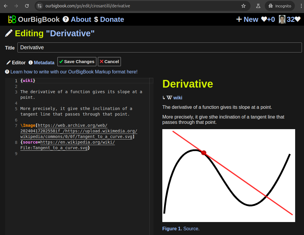
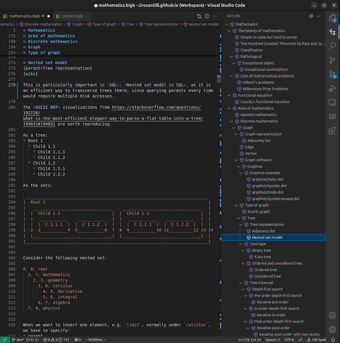
Figure 5. . You can also edit articles on the Web editor without installing anything locally. Video 3. Edit locally and publish demo. Source. This shows editing OurBigBook Markup and publishing it using the Visual Studio Code extension. 
- Infinitely deep tables of contents:

All our software is open source and hosted at: github.com/ourbigbook/ourbigbook
Further documentation can be found at: docs.ourbigbook.com
Feel free to reach our to us for any help or suggestions: docs.ourbigbook.com/#contact