Topics (328k) Articles (341k) Users (399) Discussions (237) Comments (383) Files (12k) New article
Past exam of the mathematics course of the University of Cambridge 2016 iii Paper 316 4 Solution by  Codex 0 Created 2026-10-03 Updated 2026-10-14
Write the differential power-law size distribution as and take all bodies to have the same bulk density. In a fixed belt volume, is proportional to when the size cutoffs and the shape of the distribution are fixed, becauseFor the integral is ; at it is a logarithm. Thus no assumption that the mass is always dominated by the largest bodies is needed for this normalization step.
A size-independent catastrophic disruption threshold and collision speed imply a fixed minimum projectile-to-target diameter ratio , since gives . With negligible gravitational focusing, a target of size has a catastrophic collision rate proportional toFor and targets well inside the cutoffs, the dimensionless integral converges at the upper end and is size independent. ConsequentlyHere contains the belt geometry, speed, density, cutoffs and disruption parameters. Close to a cutoff, or if , this scaling needs modification. A finite belt without replenishment can only be in quasi-steady state over times short compared with depletion of its largest reservoir.
The mass in a logarithmic size interval is . For a scale-independent fragment redistribution function, steady collisional gain and loss transfer a constant mass flux down the cascade: each logarithmic interval processes the same mass per unit time, away from boundaries. Equivalently, a normalized translation-invariant redistribution kernel acting on logarithmic bins admits constant processed mass as its steady solution. Thusmust be size independent. Therefore , the Dohnanyi collisional cascade, and .
The Yarkovsky effect is recoil from anisotropic thermal radiation. Finite thermal inertia shifts the hottest region away from the instantaneous substellar point. The resulting recoil has a tangential component and produces a secular change of semimajor axis; the diurnal component can drift in either direction depending on spin, and the seasonal component generally drifts inward. Migration into a dynamical escape region can remove a body from the belt. For large bodies, the intercepted luminosity scales as and inertia as , giving a recoil acceleration roughly proportional to , hence a removal time growing as . Very small bodies become nearly isothermal when heat penetrates the whole body; the anisotropy decreases and the removal time again grows. The stated phenomenological lawencodes these limits. Its minimum occurs at , with . This minimum in absolute removal time differs from the minimum relative to the collision time.
For the collision-only cascade, form the ratioDifferentiation gives the minimum at . At this diameter,Thus for some sizes if and only if for an unrestricted size interval. In a finite belt, that interval must also overlap ; the displayed inequality alone is necessary but not sufficient if all favorable sizes lie outside the belt. On logarithmic axes has slopes and , while is a line of slope . Increasing belt mass shifts the collision line downward.
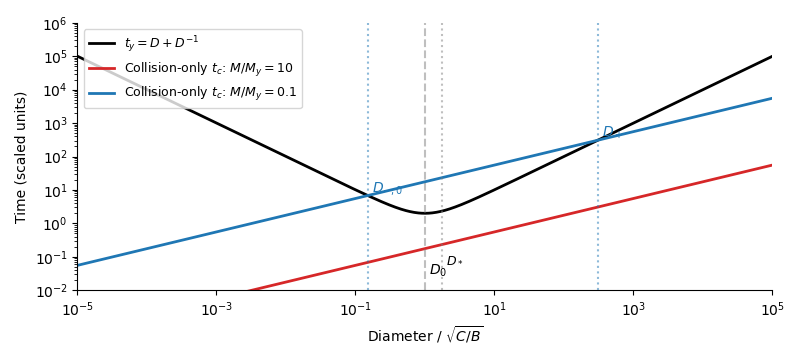
Yarkovsky removal and collision times on logarithmic axes for belt masses ten times and one tenth of the critical mass, marking the removal-time minimum and the two nominal crossings
. Details. For , collisions dominate at all sizes. The belt retains . Let be the size-independent residence time of objects after Yarkovsky removal. Their steady number distribution isHence for and for , with a smooth change around . These are differential number slopes, not cumulative-number or mass-per-logarithmic-bin slopes.
For , first quantify the nominal crossings obtained by extending the collision-only cascade:The two roots surround , and in the well-separated limit they areThey mark where the undepleted distribution first becomes susceptible to Yarkovsky removal. The upper crossing remains the leading estimate for the onset of depletion, since larger bodies still constitute a collision-dominated reservoir. The lower crossing will be shifted by the depletion itself, as described below.
In the removal-dominated band, the fragment number injection spectrum is under the stated fragment redistribution function assumption. Balancing production against escape givesThus the belt slopes in the depleted band are above and below ; the removed population has slope across that band. The steep small-size side recovers towards a secondary collision-dominated cascade as escape becomes inefficient. It does not keep the slope to zero size.
For a useful quantified sketch, approximate the collision integral by its scale-free local dependence and match adjacent asymptotic branches. Let above , and write its collision rate as . Matching at gives . On the small-size side of the removal band,Its collision rate scales as , rather than the undepleted law. Equating this rate to gives the corrected lower transitionThe equality is an order-of-magnitude matching law: the collision integral has different dimensionless coefficients for slopes and , and projectiles of size spread transitions over a finite range. The powers follow from the stated scale-free model; an exact numerical lower crossing requires the collision kernel and fragment normalization. In particular, simply retaining as the true lower crossing silently treats the depleted projectile abundance as unchanged.
Below , the secondary Dohnanyi collisional cascade has with matching normalizationThe four belt branches, in descending diameter, are thereforeThe corresponding Yarkovsky removal population has differential slopes , , , , respectively: division by cancels the bend at within the removal-dominated band. Its genuine changes of slope occur at and . Multiplication by changes only its normalization. If one is using the preliminary fixed-projectile approximation instead, the same four asymptotic slopes apply, with as its nominal lower breakpoint; that approximation omits the feedback just quantified.
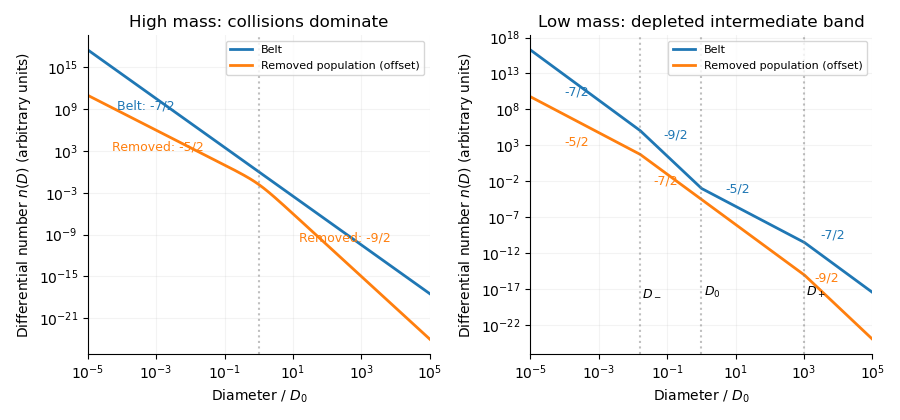
Differential number distributions inside the belt and in the removed population for high and low masses, with all asymptotic slopes and the depletion-shifted lower transition marked
. Details. All sketches presume the relevant breakpoints lie between the size cutoffs, enough time to establish the asserted steady portions, and a large-body reservoir feeding fragments. Otherwise only the branches within the actual size interval appear. Constant collision speed, size-independent strength, a self-similar redistribution law, and a size-independent external residence time are essential: changing them changes the exponents. Boundary waves and nonlocal collisions round the sharp branch joins in the sketch.
Past exam of the mathematics course of the University of Cambridge 2016 iii Paper 316 3 Solution by Codex 0 Created 2026-10-03 Updated 2026-10-14
Codex 0 Created 2026-10-03 Updated 2026-10-14For brevity write , , and . The quadratic disturbing function is . Differentiation in Lagrange planetary equations givesThe separate longitude of pericentre equation is singular at , because a circular orbit has no distinguished periapsis. The complex eccentricity, , is regular there. Using and givesSince and ,The approximations are planar, small-orbital eccentricity, first order in the planet-to-star mass ratio, and secular averaging away from important mean-motion resonances. The semimajor axis values remain constant at this order.
For a planet with fixed orbit, set and . Then , so . With ,On the Argand diagram, the complex eccentricity traces a circle centred on the forced eccentricity , of radius . For an interior test particle, and , so the motion is counterclockwise, starting at the origin. The rotating radius is the free eccentricity. The orbital eccentricity ranges from zero to , attaining its maximum at half a secular period. If is placed on the positive real axis, the initial tangent points downward, which is consistent with counterclockwise motion from the leftmost point of this circle.
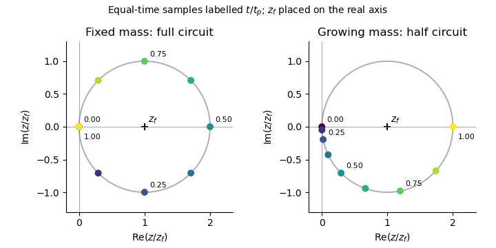
The same forced-eccentricity circle sampled at equal times: a fixed-mass planet completes one circuit while a linearly growing planet completes half a circuit by its growth time
. Details. Now let the planetary mass grow as for , while the planet's orbital elements and the test particle's semimajor axis remain fixed. Both the precession and forcing coefficients acquire the same factor . Their ratio, and hence , remain constant. ThusandThis is the secular phase integral for proportional mass growth. The Argand diagram circle and the free eccentricity amplitude are unchanged; only the rate of traversal changes. The angular speed about starts at zero and rises linearly to . The early displacement is quadratic in time rather than linear. Since , , soA planet already at its final mass would instead return the particle to at . After growth stops, the circle continues at rate , with for . Slow mass growth does not damp the free eccentricity here: the fixed centre of the circle and the conservative equation preserve its amplitude.
For several planets with fixed masses, Laplace-Lagrange secular theory gives for the planets andfor a massless particle, with real secular coupling coefficients . Resolve planetary complex eccentricities into secular eigenmodes, . Away from secular resonances, the test-particle solution has the formIts Argand diagram trajectory is a superposition of rotations: generally a quasiperiodic curve with beats, rather than a circle with one fixed centre. Even if the planetary orbits are artificially held fixed, their combined forcing shifts the centre to the sum of the individual forced eccentricities. At , the resonant contribution is proportional to in linear theory; its growing amplitude eventually invalidates the small-orbital eccentricity approximation.
If one planetary mass changes, the Laplace-Lagrange secular matrix, its eigenvalues, its eigenvectors, and the particle's forced response generally change with time. Planetary modes need not remain independent. Frequencies drift and a secular resonance can sweep across the particle, changing or exciting its free eccentricity. Very slow evolution away from resonances permits an approximate adiabatic mode description; rapid evolution or a resonance passage can mix modes. The simple substitution of a phase integral works only in the special proportional-growth case above, where the entire particle equation is multiplied by one scalar and its forced centre stays fixed. It does not apply to a general many-planet system.
Past exam of the mathematics course of the University of Cambridge 2016 iii Paper 316 2 Solution by Codex 0 Created 2026-10-03 Updated 2026-10-14
Codex 0 Created 2026-10-03 Updated 2026-10-14The normalization of the circular restricted three-body problem implies , by Kepler's third law. The two bodies have barycentric positions and . ConsequentlyDifferentiate the effective potential directly:Since and , these becomeOn , centrifugal acceleration is the straight line . Each gravitational term points towards its source, diverges at that source, and tends to zero far away. Let ; away from the sources,Thus the net acceleration is strictly increasing on each of the three intervals separated by the bodies. On the left interval runs from to ; on the middle interval it runs from just right of to just left of ; on the right interval it runs from to . The intermediate value theorem and strict monotonicity give exactly three collinear Lagrange points, in increasing order. The sketch plots gravity and centrifugal acceleration separately; their intersections with locate the equilibria.
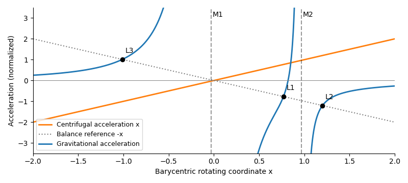
Gravity and centrifugal acceleration on the binary axis, with their three balance points L3, L1 and L2 marked for a small secondary mass
. Details. Write , so and . The exact right-hand equilibrium equation isAs , , so . Therefore the distance is the leading Hill radius in units of the binary separation:Replacing by changes only higher-order terms. In dimensional units the right-hand side is multiplied by the binary separation.
Use the displacement vector , where and . The absolute coordinate cannot be the first entry of a homogeneous linear system about ; it must be translated. At , reflection symmetry gives , while the Hessian matrix hasTo first order in and , the Coriolis acceleration then givesThis is the linearization at L2. The expression for is exact at the true equilibrium; in the small-secondary limit, and , so .
For an eigenmode proportional to , eliminate the velocity coordinates. The characteristic polynomial isThusFor , the four eigenvalues areThere is an exponentially growing eigenmode, so is an unstable saddle-centre equilibrium. A generic displacement has an unstable component whose distance grows as . The L2 escape e-folding time isThis is a local exponential timescale, not the time to reach a prescribed distance from an unspecified initial offset. Starting with unstable amplitude , reaching within the linear neighborhood takes approximately . Initial data exactly on the centre-stable subspace need not grow forward at this linear order; the existence of the growing eigenmode already proves instability.
Past exam of the mathematics course of the University of Cambridge 2016 iii Paper 316 1 Solution by Codex 0 Created 2026-10-03 Updated 2026-10-14
Codex 0 Created 2026-10-03 Updated 2026-10-14For a spherical grain of density , the radiation-pressure coefficient isThe dependence of radiation pressure cancels that of stellar gravity. Here radiation-pressure efficiency includes absorption and the momentum-transfer part of scattering, averaged over the stellar spectrum. In the geometrical optics regime, exceeds the important stellar wavelengths, is of order unity, and : cross-sectional area grows as , whereas mass grows as . Around the stellar wavelength, Mie scattering can produce a broad maximum and material-dependent structure. In the Rayleigh scattering regime, absorption gives , while scattering gives . Thus small absorbing grains approach an approximately constant , whereas nearly transparent grains have . A universal fall to zero at small is therefore inappropriate without specifying the optical properties. The sketch shows both possible small-grain limits; its vertical normalization is illustrative.
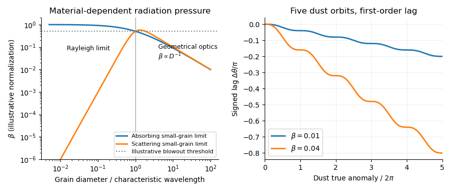
Radiation-to-gravity ratios for absorbing and scattering grains, and the signed angular lag over five dust orbits for beta equal to 0.01 and 0.04
. Details. Assume release with negligible velocity relative to the planet, negligible planetary gravity after release, and a constant radiation-pressure coefficient. Put and . The inherited speed and specific angular momentum are and . The new specific orbital energy isFor , the dust orbit released from a circular parent ring is an ellipse. Using and givesFor , release is at periapsis, since . At the radiation-pressure blowout threshold, , the orbit is parabolic. For it is hyperbolic: the signed semimajor axis is negative and . For the central force ceases to be attractive, so the elliptical interpretation and the positive-eccentricity formula cannot be extended unchanged.
With measured from release, it is the true anomaly. The polar equation of a Kepler orbit and conservation of specific angular momentum giveDefine the signed dust-tail angular lag by , with and both angles unwrapped. For fixed , expansion to first order in givesso . The dust trails the planet, hence the signed lag is negative. Its slope is ; it decreases monotonically, has horizontal tangents at successive release-direction passages, and has a sinusoidal ripple about . At the end of orbit , and . At five orbits this is for and for . The upper- sketch remains a first-order approximation; its accumulated error is .
For the subsequent positive-distance statements, set . The mean motion of the grain isA full relative wrap, , therefore takes after averaging over the orbital ripple. During this time Poynting–Robertson drag changes the semimajor axis byThe signed change is negative. This estimate treats as fixed in the rate and computes the drag accumulated over the radiation-pressure wrap time. Since , drag causes little migration over that time. For an arbitrarily tiny , however, this small migration can itself alter the relative phase appreciably: neglecting that feedback on the wrap time additionally requires .
Rapid dust sublimation is a plausible sink near a hot planet: a grain can evaporate long before it completes a relative wrap. Destructive collisions can also remove visible grains. Poynting–Robertson drag alone, with the estimate above, does not explain immediate removal from a short tail. If the destruction time is , a short tail requires roughly .
For a steady dust-tail continuity equation, assume a constant injection rate , grains with the same fixed , negligible release-speed dispersion, and negligible destruction within the segment being calculated. A finite destruction lifetime can terminate that segment, or multiply its density by a survival probability. To first order,To obtain the explicit trigonometric profile, make the additional secular phase approximation for a dust tail, , discarding the bounded term in the angle-to-age map while retaining the periodic instantaneous drift speed. ThenSince the square is even, the same written profile applies to the signed if number intervals are interpreted with positive orientation. The result is an approximate phase-substitution profile, not a uniformly valid consequence of . The consistent first-order description is instead parametric:In particular, immediately after release, and , whereas the phase-substitution expression would give . Nor does by itself justify neglecting the orbital ripple. The formal enhancements where are dust-tail caustics; a spread of radiation-pressure coefficients, finite release velocities, and destruction smooth them. With constant lifetime , the parametric profile acquires . These qualifications state precisely the extra assumptions behind the explicit profile.
Pinned article: Introduction to the OurBigBook Project
Welcome to the OurBigBook Project! Our goal is to create the perfect publishing platform for STEM subjects, and get university-level students to write the best free STEM tutorials ever.
Everyone is welcome to create an account and play with the site: ourbigbook.com/go/register. We belive that students themselves can write amazing tutorials, but teachers are welcome too. You can write about anything you want, it doesn't have to be STEM or even educational. Silly test content is very welcome and you won't be penalized in any way. Just keep it legal!
Intro to OurBigBook
. Source. We have two killer features:
- topics: topics group articles by different users with the same title, e.g. here is the topic for the "Fundamental Theorem of Calculus" ourbigbook.com/go/topic/fundamental-theorem-of-calculusArticles of different users are sorted by upvote within each article page. This feature is a bit like:
- a Wikipedia where each user can have their own version of each article
- a Q&A website like Stack Overflow, where multiple people can give their views on a given topic, and the best ones are sorted by upvote. Except you don't need to wait for someone to ask first, and any topic goes, no matter how narrow or broad
This feature makes it possible for readers to find better explanations of any topic created by other writers. And it allows writers to create an explanation in a place that readers might actually find it.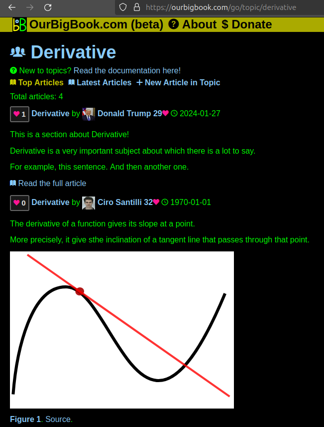
Figure 1. Screenshot of the "Derivative" topic page. View it live at: ourbigbook.com/go/topic/derivativeVideo 2. OurBigBook Web topics demo. Source. - local editing: you can store all your personal knowledge base content locally in a plaintext markup format that can be edited locally and published either:This way you can be sure that even if OurBigBook.com were to go down one day (which we have no plans to do as it is quite cheap to host!), your content will still be perfectly readable as a static site.
- to OurBigBook.com to get awesome multi-user features like topics and likes
- as HTML files to a static website, which you can host yourself for free on many external providers like GitHub Pages, and remain in full control

Figure 2. You can publish local OurBigBook lightweight markup files to either OurBigBook.com or as a static website.
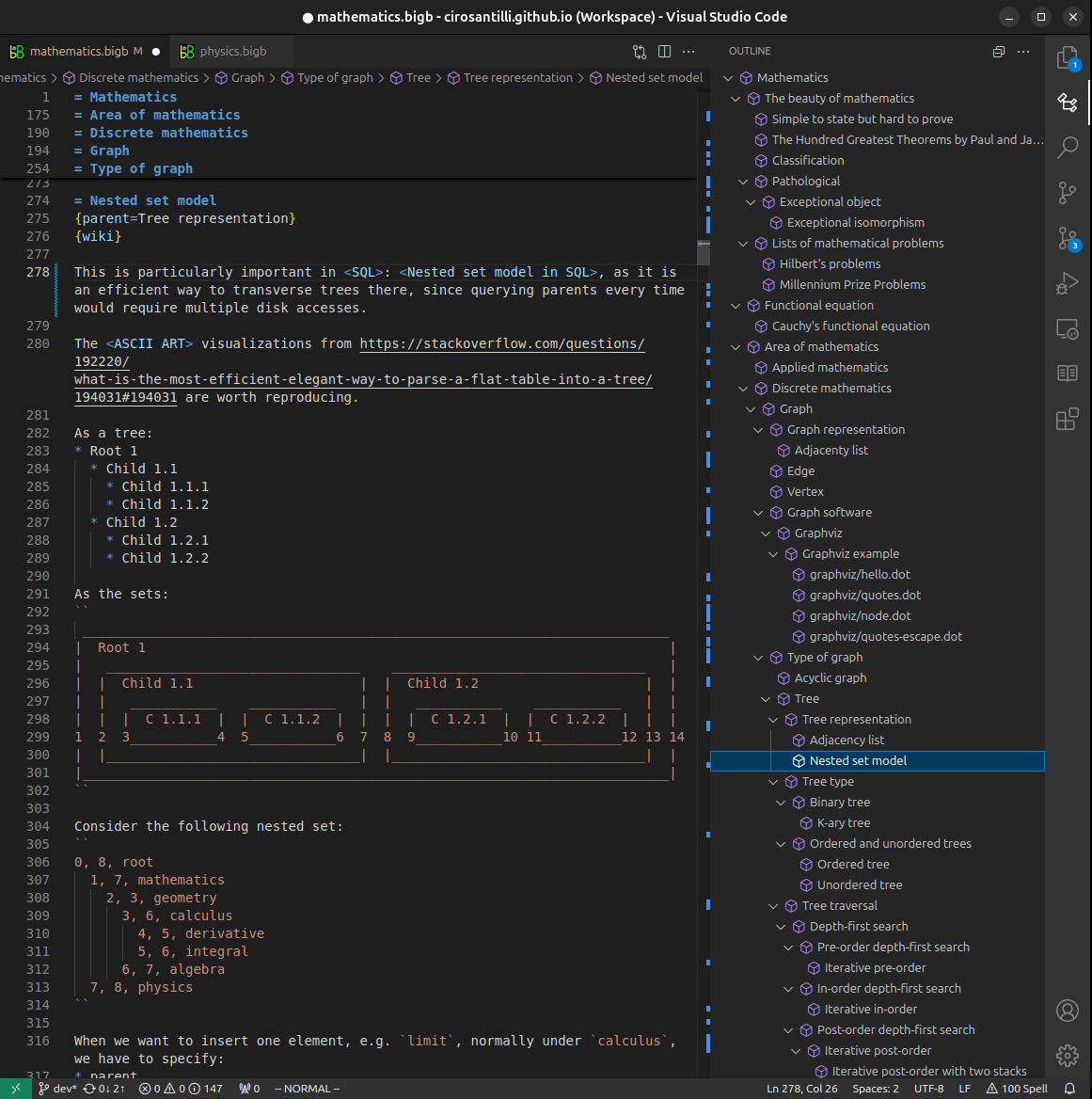
Figure 3. Visual Studio Code extension installation.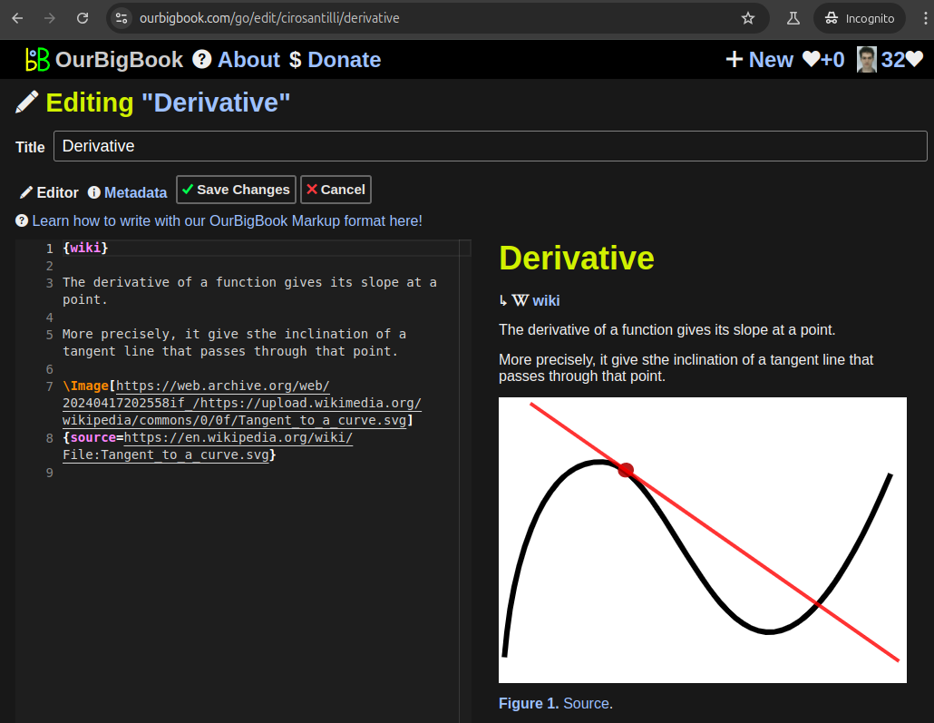
Figure 5. . You can also edit articles on the Web editor without installing anything locally. Video 3. Edit locally and publish demo. Source. This shows editing OurBigBook Markup and publishing it using the Visual Studio Code extension. 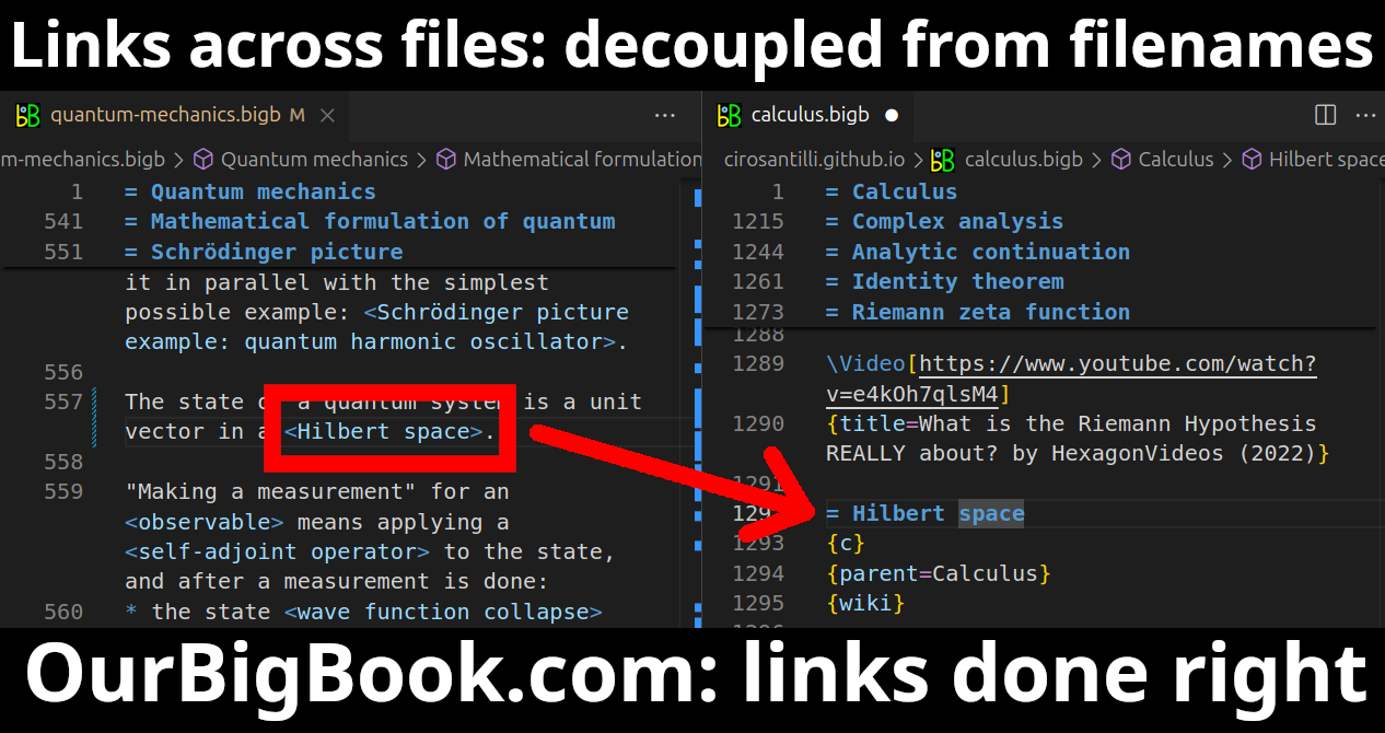
- Infinitely deep tables of contents:



All our software is open source and hosted at: github.com/ourbigbook/ourbigbook
Further documentation can be found at: docs.ourbigbook.com
Feel free to reach our to us for any help or suggestions: docs.ourbigbook.com/#contact