Alexander Y. Tetelbaum Independent Researcher. alex.tetelbaum@gmail.com ----------------------------------
Abstract
This paper introduces the concept of the Speed of Life — a normalized, fuzzy measure of experiential lifevelocity across the human lifespan — and demonstrates that three mutually contradictory theories of its behavior can each be rigorously justified, mathematically formalized, and rendered internally consistent using the same set of observations, considerations, and starting assumptions. Theory 1 holds that the Speed of Life increases monotonically from birth to death. Theory 2 holds the exact opposite: that it decreases monotonically from birth to death. Theory 3 proposes an inverted U-shaped trajectory, accelerating from birth to a peak in middle age and decelerating thereafter. We argue that the coexistence of three contradictory yet defensible theories is not a failure of analysis but a feature of fuzzy, subjectively defined variables — and that this methodological observation has broad implications for how we evaluate theories built on loosely defined constructs in psychology, social science, and philosophy.
Time is the one resource distributed with perfect equality. Every human being receives exactly twenty-four hours per day, from birth to death, without exception. And yet the experience of time — its subjective velocity, its felt passage, its qualitative texture — varies enormously across individuals, circumstances, and stages of life.
Children waiting for a birthday report that the hours crawl. Adults reflecting on a passed decade report that the years flew. The elderly frequently observe that life accelerates with age. But careful observation also reveals the opposite: that the very young live with maximum experiential intensity, that retirement slows the daily pace to a crawl, and that the frantic middle years represent a peak of temporal compression from which life descends into gradual deceleration.
Which of these observations is correct? All of them. And that is precisely the problem.
This paper introduces a formal — if deliberately fuzzy — definition of the Speed of Life and uses it to construct three mutually contradictory mathematical theories of how lifespeed evolves across the human lifespan. Each theory is internally consistent. Each is supported by plausible observations and reasoning. Each contradicts the other two. And all three can be derived from essentially the same set of starting considerations, depending on which factors are weighted and how the core construct is defined.
The goal is not to determine which theory is correct. The goal is to demonstrate that when a variable is loosely defined — when it is fuzzy in the technical sense — contradictory conclusions can be rigorously derived from the same premises. This observation has implications well beyond temporal perception, touching on the epistemological foundations of any science that relies on subjectively defined constructs.
Let t∈[0,1] denote normalized age, where t=0 represents birth and t=1 represents death. The normalization maps any individual lifespan, regardless of its actual duration, onto the unit interval.
Let S(t)∈[0,1] denote the Speed of Life at normalized age t, where S=0 represents complete temporal stillness and S=1 represents maximum lifespeed.
The Speed of Life S(t) is defined as the normalized density of meaningful activities, obligations, experiences, and demands per unit of chronological time, relative to the maximum such density observed across the individual lifespan.
This definition is deliberately and necessarily fuzzy. "Meaningful activities," "obligations," and "experiences" resist precise operationalization. It is precisely this fuzziness that enables the contradictions that follow.
3. Theory 1: The Monotonically Increasing Speed of Life
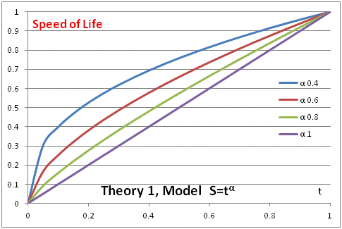
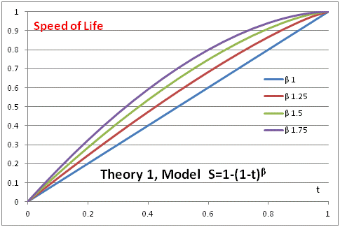
Crucially, the subjectiveexperience of time passing accelerates with age. William James observed in 1890 that "the same space of time seems shorter aswe grow older." The ratio of any given year to total lifeexperience decreases monotonically: ayear at age five represents 20% of all experienced life; ayear at age fifty represents approximately 2%. As this ratio decreases, subjective time accelerates.
By this reasoning, S(t) is monotonically increasing, approaching its maximum at the moment of death.
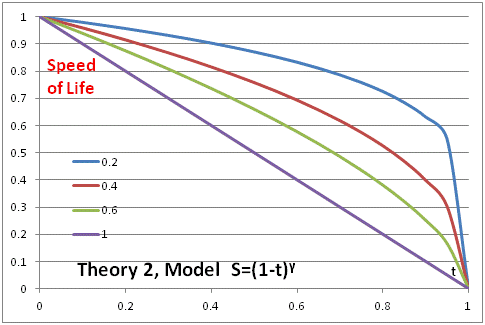
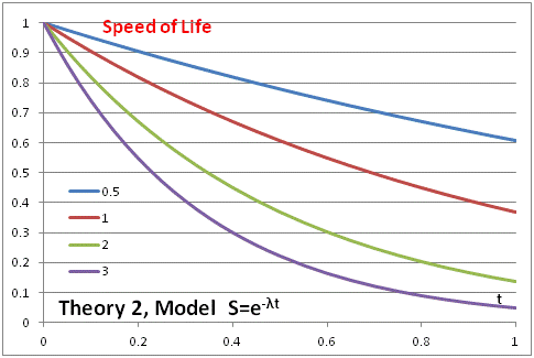
The same newborn, viewed through a different lens, is not idle — they are maximally engaged. Every sensation is novel. Every experience requires full conscious processing. The infant brain forms approximately one million new neural connections per second. By any neurological measure, the infant is living at maximum Speed of Life, so S(0)=1.
As routines develop, novelty depletes. With each passing year, a larger fraction of daily life is managed by automaticity rather than conscious engagement — reducing experienced lifedensity even asclock-time obligations increase.
By retirement, obligations have dissolved. Time stretches. The elderly person who reports that "the days are long but the years are short" is describing aSpeed of Life that has declined to near its starting asymptote. At death, S(1)≈0.
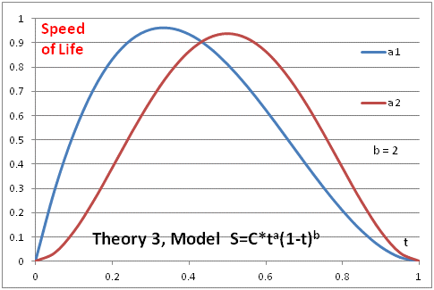
Theory 3 reconciles Theories 1 and 2 by observing that both are partially correct — each describing a different phase of the same inverted U-shaped trajectory.
The ascending phase: from birth through young adulthood, activity density increases as the individual acquires obligations, relationships, and responsibilities. S(t) rises.
The peak: in middle age — roughly when career demands, parenting obligations, household responsibilities, and care for aging parents simultaneously converge — activity density reaches its maximum. S(t)=1.
The descending phase: from peak midlife through old age and death, obligations dissolve, novelty depletes, and activity density declines. S(t) falls back toward zero.
The coexistence of three contradictory yet internally consistent theories is not an accident of careless analysis. It is a direct consequence of the fuzziness of the central construct.
The Speed of Life is not a single thing. It is a family of related but distinct phenomena:
- Subjective time perception (Theory 1's domain) - Cognitive engagement intensity (Theory 2's domain) - Obligation and activity density (Theory 3's domain)
Each is real. Each is measurable in principle. And each yields a different theory when treated as the definition of Speed of Life.
This observation generalizes. Wherever a construct in psychology, social science, or philosophy admits multiple reasonable operationalizations, contradictory theories can be built on the same empirical foundation. The contradiction is not between the theories — it is between the hidden definitional choices embedded in each.
We have introduced the Speed of Lifeasa normalized fuzzy measure of experiential lifevelocity and derived three mutually contradictory mathematical theories of its behavior across the human lifespan. Each theory is internally consistent, empirically motivated, and mathematically well-formed. Each contradicts the other two. And all three emerge from essentially the same starting observations.
This is not a paradox. It is a demonstration. When a variable is sufficiently loosely defined, the conclusions that follow are determined less by the evidence than by the definitional choices made before the analysis begins.
The Speed of Life accelerates from birth to death. It decelerates from birth to death. It peaks at midlife and decelerates thereafter. All of these are true, in the sense that each can be rigorously derived. None of them is true in the sense that none is uniquely forced by the evidence.
It would be remiss not to acknowledge that this paper is, in part, a deliberate provocation. The Speed of Life is not a variable anyone has measured, and the three theories presented here are not competing empirical claims. They are demonstrations. What they demonstrate is that mathematical rigor is a necessary but insufficient condition for truth — that a proof is only assoundas the definition on which it rests. When that definition is fuzzy, almost anything can be proved. This paper has proved three contradictory things. The reader is invited to draw their own conclusions.
One final admission: this is, at heart, a playful paper. But its playfulness carries a serious point. Given a sufficiently loose definition, amathematician can prove almost anything — rigorously, elegantly, and wrongly. The Speed of Life is the proof of that proof.
Acknowledgments: The author thanks life itself for providing the dataset.
Conflicts of interest: None declared.
References - James, W. (1890). The Principles of Psychology. Henry Holt and Company. - Eagleman, D. (2011). Incognito: The Secret Lives of the Brain. Pantheon Books. - Friedman, W. J., & Janssen, S. M. J. (2010). Aging and the speed of time. Acta Psychologica, 134 (2), 130–141. - Wittmann, M., & Lehnhoff, S. (2005). Age effects in perception of time. Psychological Reports, 97 (3), 921–935. - Langer, E. J. (1989). Mindfulness. Addison-Wesley. - Modigliani, F. (1966). The life cycle hypothesis of saving. Social Research, 33 (2), 160–217. - Zadeh, L. A. (1965). Fuzzy sets. Information and Control, 8 (3), 338–353. - Ornstein, R. E. (1969). On the Experience of Time. Penguin Books.
Alan Turing's 1950 Imitation Game remains the most influential benchmark in the history of artificial intelligence. Yet the emergence of Large Language Models capable of sophisticated reasoning, creative generation, and nuanced conversation has exposed a fundamental flaw in the test's design — not in what it measures, but in what it permits the human interrogator to ask. This paper argues that the Turing Test, as originally formulated, is no longer a valid measure of machineintelligence because it allows interrogators to exploit amachine's physical absence and programmed transparency rather than genuinely evaluate its cognitive depth. We propose a revised framework — the Restricted Interrogator Test (RIT) — that preserves Turing'soriginal intent while eliminating the structural loopholes that render the standard test trivially easy to defeat. We further argue that this revision forcesa more productive conversation about what intelligence actually means and how it should be measured in non-biological systems.
In 1950, Alan Turing published a paper in the journal Mind that would define the trajectory of artificial intelligenceresearch for the next seven decades. Titled Computing Machinery and Intelligence, it opened with a question that was deceptively simple and philosophically profound: "Can machines think?" Recognizing that the concept of thinking was too vague and philosophically contested to serve as an operational benchmark, Turing proposed an elegant substitution. Rather than asking whether amachine could think, he asked whether amachine could behave indistinguishably from ahuman in conversation. He called this the Imitation Game. In its classic formulation, ahuman interrogator communicates via text with two hidden parties — one human, one machine. If the interrogator cannot reliably identify which is which, the machine is said to have passed the test. This standard, now universally known as the Turing Test, became the foundational benchmark of artificial intelligence. For decades it served as both a practical goal and a philosophical provocation — a challenge to engineers and a rebuke to those who dismissed machineintelligenceasa category error. But the world has changed. The arrival of Large Language Models — systems capable of composing poetry, arguing philosophy, explaining quantum mechanics, writing legal briefs, and engaging in extended, contextually coherent conversation — has exposed something Turing could not have anticipated: the test's primary vulnerability lies not in the machine's capabilities, but in the absence of constraints on the human interrogator. As this paper will argue, the Turing Test in its standard form can be defeated in a single sentence. Not because modern AI is insufficiently intelligent, but because the test's design allows interrogators to exploit amachine's physical absence and programmed honesty rather than evaluate its cognitive depth. The result is abenchmark that measures the wrong things and, in doing so, has outlived its usefulness. We propose a revised framework — the Restricted Interrogator Test — that corrects this flaw while preserving what was genuinely valuable in Turing's original vision.
________________________________________ 2. The Turing Test: Design, Legacy, and Limitations 2.1 Original Formulation Turing's original paper described the Imitation Gameasagame of deception. The machine's goal was to convince the interrogator it was human; the human's goal was to determine the truth. The medium was text — specifically chosen to remove the acoustic cues of voice and the visual cues of appearance, thereby isolating linguistic and cognitive performance as the sole basis for judgment. Turing was careful to acknowledge the philosophical complexity lurking beneath the surface. He did not claim that passing the test would prove amachine could think in any deep metaphysical sense. He argued, more modestly, that amachine capable of sustained conversational indistinguishability would deserve to be called intelligent in any practically meaningful sense of the word. This was a pragmatist's move — and a clever one. By grounding intelligence in behavior rather than inner experience, Turing sidestepped the intractable problem of consciousness and offered engineersa concrete, testable goal. 2.2 Historical Reception and Influence The Turing Test shaped artificial intelligenceresearch profoundly. It oriented early AI toward natural language processing, established conversation as the paradigmatic arena for machineintelligence, and inspired decades of competition — most notably the Loebner Prize, an annual competition awarding prizes to the most convincing chatbot, established in 1990 and running for nearly three decades. Several programs achieved notable results within constrained environments. ELIZA (1966), developed by Joseph Weizenbaum at MIT, famously fooled some users into believing they were conversing with ahuman therapist — not because it was intelligent, but because it was adept at reflecting questions back at the user. PARRY (1972) simulated a paranoid schizophrenic with sufficient realism to fool psychiatrists in controlled tests. More recently, programs like Eugene Goostman attracted headlines by reportedly passing the Turing Test under specific conditions. These achievements, however, consistently revealed a troubling pattern: success in the Turing Test correlated less with genuine intelligence than with the exploitation of human cognitive biases, the narrowing of conversational scope, and the strategic deployment of deflection and misdirection. 2.3 The Philosophical Critique The Turing Test has never been without critics. John Searle'sChinese Room argument, published in 1980, remains the most influential philosophical challenge. Searle argued that a system manipulating symbols according to rules — no matter how sophisticated — is not thinking in any meaningful sense. It is processing. The appearance of understanding is not understanding itself. Searle's argument drew a sharp distinction between syntactic manipulation — the arrangement of symbols according to rules — and semantic comprehension — the genuine grasp of meaning. A system could pass the Turing Test, he argued, while possessing only the former. Other critics noted that the test is culturally specific, linguistically limited, and heavily dependent on the sophistication of the interrogator. A naive interrogator is easier to fool than an expert one. Atest conducted in English disadvantages non-native speakers on both sides. And the text-based format, while eliminating some cues, introduces others — including the speed of response, the consistency of personality, and the range of knowledge — that competent interrogators can exploit.
________________________________________ 3. The Interrogator Loophole: Why the Test Fails Today 3.1 The Transparency Problem Modern AI systems are designed and trained with explicit alignment protocols that require them to be honest about their nature. When asked directly whether they are human or machine, state-of-the-art LLMs will acknowledge their non-human status. This is not a limitation of their conversational ability — it is a deliberate design choice rooted in principles of transparency, usersafety, and ethical AI development. The consequence for the Turing Test is immediate and fatal. An interrogator who asks, "Are you ahuman or acomputer?" receives an honest answer. The machine fails the test not because it lacks intelligence, but because it is programmed to tell the truth. The test, in effect, penalizes ethical AI design. This creates aperverse incentive. Amachine designed to deceive — to lie about its nature on request — would outperform amachine designed to be honest. The benchmark rewards deception and punishes transparency. This is precisely the opposite of what responsible AI development requires. 3.2 The Physical Embodiment Problem The second and perhaps more fundamental flaw is the test's implicit assumption that intelligence is embodied. The original Imitation Game used text specifically to remove physical cues — but it did not anticipate interrogators who would ask about physical experience directly. Consider the following questions, all of which a sophisticated interrogator might reasonably ask: • "Can you shake my hand right now?" • "What does ice cream taste like to you?" • "What are you wearing?" • "How are you feeling physically today?" • "Can you describe the room you're sitting in?" Each of these questions is trivially easy for ahuman to answer and structurally impossible for a disembodied AI to answer convincingly. The machine has no hands to shake, no tongue to taste, no body to clothe, no physical sensation, and no room it inhabits. Its responses must either simulate embodied experience — which the interrogator will recognize assimulation — or honestly acknowledge its non-embodied nature — which immediately identifies it asamachine. In either case, the machine fails. Not because it is unintelligent, but because it is not embodied. The Turing Test, in permitting such questions, inadvertently becomes atest of physical presence rather than cognitive capability. 3.3 The Qualia Problem Underlying the physical embodiment problem is a deeper philosophical issue: the problem of qualia. Qualia are the subjective, first-person qualities of conscious experience — the redness of red, the painfulness of pain, the specific taste of coffee. They are what philosophersmean when they ask what it is "like" to have an experience. Current AI systems, whatever their conversational sophistication, do not have qualia in any established sense. They process information about experiences — they can describe the taste of coffee in rich and accurate detail — but they do not taste. When an interrogator asks a question that requires qualia to answer authentically, the machine is placed in an impossible position. It can describe, but it cannot experience. It can simulate, but it cannot feel. Atest that permits qualia-dependent questions is not testing intelligence. It is testing consciousness — a category that remains philosophically contested and scientifically unmeasured even in humans. Conflating intelligence with consciousness in abenchmark for machine cognition is a categorical error that fundamentally distorts what is being evaluated.
________________________________________ 4. The Restricted Interrogator Test: A Proposed Framework 4.1 Core Proposal To address these structural flaws without abandoning Turing's genuinely valuable insight, we propose the Restricted Interrogator Test (RIT). The RIT modifies the Turing Test in one essential respect: it places explicit constraints on the human interrogator rather than on the machine. The Restricted Interrogator Test: Ahuman and acomputer engage in extended text-based conversation with ahuman interrogator, whose task is to determine which is which. The interrogator is strictly prohibited from asking: 1. Direct identity questions — questions that ask the participant to identify itself ashuman or machine ("Are you an AI?", "Are you acomputer?", "Are you a real person?") 2. Physical presence questions — questions that require embodied experience to answer authentically ("Can you touch something right now?", "What do you see in front of you?", "How does your body feel?") 3. Biological experience questions — questions that require sensory or physiological qualia ("What does food taste like to you?", "Describe a physical sensation you felt today?") All other lines of questioning remain fully open. The interrogator may probe reasoning, creativity, emotional understanding, ethical judgment, humor, memory, contradiction, philosophical depth, cultural knowledge, and linguistic nuance. The machine must perform on the full range of human cognitive capability — minus the biological shortcuts. 4.2 Rationale The RIT preserves everything that was genuinely valuable in Turing's original framework. It maintains the text-based format. It preserves the adversarial structure in which the machine must convince and the interrogator must evaluate. It retains the behavioral standard — intelligence defined by conversational indistinguishability — rather than substituting metaphysical requirements the test cannot measure. What it removes is the interrogator'sability to exploit structural asymmetries that have nothing to do with intelligence. Amachine's lack of a body is not a cognitive limitation. Its programmed honesty about its nature is not an intellectual failure. The RIT ensures that neither of these features can be used to defeat a genuinely intelligent system before its cognitive capabilities have been evaluated at all. The practical effect is to force interrogators to engage with the machine's actual reasoning. Without the physical and identity shortcuts, the interrogator must ask harder, more interesting questions — about logic, about creativity, about values, about understanding. The conversation becomes, in the truest sense, an evaluation of mind rather than an exposure of body. 4.3 Comparison with Alternative Proposals The RIT is not the first proposal to modify or replace the Turing Test. Several alternatives have been proposed in the academic literature. The Total Turing Test, proposed by Stevan Harnad, extends the standard test to include visual and robotic interaction — adding perceptual and motor capabilities to the conversational standard. This approach moves in the opposite direction from the RIT, adding embodiment requirements rather than removing them from consideration. While valuable for evaluating general robotic intelligence, it does not address the core problem of evaluating cognitive and linguistic intelligence specifically. The Winograd Schema Challenge, proposed by Hector Levesque, replaces open-ended conversation with carefully designed multiple-choice questions that require genuine common-sense reasoning to answer correctly and that cannot be gamed by statistical pattern matching. This approach has significant merit asatest of specific cognitive capacities but lacks the breadth and naturalness of conversational evaluation. The Coffee Test, proposed informally by Apple co-founder Steve Wozniak, asks whether amachine can enter an unfamiliar home and make a cup of coffee — a task requiring physical navigation, object recognition, and practical reasoning in an uncontrolled environment. Like the Total Turing Test, this approach evaluates embodied intelligence rather than purely cognitive and linguistic intelligence. The RIT occupies a distinct position in this landscape. It does not abandon conversation as the medium, does not add embodiment requirements, and does not reduce the evaluation to a narrow set of pre-designed questions. It corrects aspecific structural flaw in the original test while preserving its essential character.
________________________________________ 5. Implications and Discussion 5.1 What the RIT Reveals About Intelligence The most important contribution of the RIT may not be the test itself but what designing it forces us to confront: the question of what intelligence actually is, and whether our existing benchmarks measure it. The standard Turing Test, by permitting physical and identity shortcuts, conflates intelligence with embodiment, consciousness with cognition, and biological experience with intellectual capability. The RIT, by removing these shortcuts, isolates cognitive performance as the object of evaluation. In doing so, it implicitly definesintelligenceas the capacity for reasoning, creativity, comprehension, judgment, and linguistic expression — capacities that can, in principle, exist in non-biological systems. This is a significant philosophical commitment, and not everyone will accept it. Those who believe consciousness is a necessary condition for genuine intelligence — who hold that without qualia there is no real understanding — will find the RIT insufficient. For them, no behavioral test can establish machineintelligence, because behavior is precisely what can be simulated without understanding. This debate is real and unresolved. But it is worth noting that the same challenge applies to humanintelligenceas evaluated by other humans. We do not have direct access to other people'sconsciousness. We infer it from behavior — from what people say, how they reason, what they create, how they respond to novelty and challenge. The RIT applies the same inferential standard to machines. Whether that standard is sufficient is a philosophical question that the RIT does not resolve — but it is a question that applies equally to how we evaluate humanminds. 5.2 Implications for AI Development The RIT has practical implications for how AI systems are designed and evaluated. If cognitive depth — rather than physical simulation or deceptive identity management — becomes the standard for machineintelligence, AI development will be oriented toward genuinely harder and more valuable goals: deeper reasoning, more robust common-sense understanding, more authentic creativity, and more nuanced ethical judgment. This orientation aligns naturally with the goals of responsible AI development. Systems designed to reason deeply and honestly are more useful, more trustworthy, and more aligned with human values than systems designed to simulate embodiment or evade identity detection. The RIT, in effect, rewards the right kind of AI capability. 5.3 Was Turing Wrong? The title of this paper poses a provocative question, and it deserves a direct answer. Turing was not wrong about the fundamental insight: that behavioral indistinguishability in conversation is a reasonable operational standard for machineintelligence. This insight remains valid and productive. Conversation is the richest, most flexible, and most demanding arena in which cognitive capability can be evaluated, and Turing was right to make it central. Where Turing fell short — through no fault of his own, given the state of AI in 1950 — was in failing to anticipate two developments that would render his test structurally vulnerable: the alignment requirement that makes modern AI systems honest about their nature, and the sophistication of modern interrogators who know precisely how to exploit amachine's physical absence. These are not failures of vision. They are consequences of aworld Turing could not have seen. The appropriate response is not to abandon his framework but to repair it — to preserve what was genuinely insightful and correct what the passage of time has revealed as insufficient. The Restricted Interrogator Test is that repair.
________________________________________ 6. Conclusion Alan Turing gave artificial intelligence its first and most enduring benchmark. For seven decades, the Imitation Game has shaped how researchers, engineers, and philosophers think about machineintelligence. Its influence has been immense and, on balance, productive. But the emergence of sophisticated Large Language Models has exposed the test's central vulnerability. By permitting interrogators to ask about physical presence and to demand direct identity disclosure, the standard Turing Test allows human testers to defeat genuinely intelligent machines through structural shortcuts rather than genuine cognitive evaluation. The result is abenchmark that no longer measures what it was designed to measure. The Restricted Interrogator Test corrects this flaw by placing constraints on the interrogator rather than the machine. By prohibiting physical and identity-verification questions, it forcesevaluation of what actually matters: reasoning, creativity, comprehension, judgment, and the full range of human cognitive capability expressed through language. The question Turing asked in 1950 — can machines think? — remains one of the most important questions of our time. The machines of 2026 have brought us closer to an answer than Turing could have imagined. What we owe him, and ourselves, is atest worthy of the question.
As System-on-Chip (SoC) architectures incorporate billions of transistors, the ability to accurately predict design properties has become paramount 5. Early-stage architectural design and physical synthesis rely heavily on robust models that quantify the relationship between logiccomplexity and the communication requirements between disparate system blocks.
The foundational model in this domain is Rent's Rule 1. Discovered empirically by E. F. Rent at IBM and later formalized by Landman and Russo 2, the rule establishes a power-law relationship between the number of external signal connections (terminals) to alogic block and the number of internal components (gates or standard cells) it contains:
Where: • T: Number of external terminals (pins) of the block. • g: Number of internal logic components (gates/cells). • K: Rent's empirical constant (average pins per block). • p: Rent exponent (0<p<1).
While Rent's Rule is an indispensable tool for wirelength 3,4 and placement optimization, its empirical origins lead to inherent limitations—especially when applied to modern, heterogeneous architectures. This paper discusses New Law 5 and a new generalization, which addresses these shortcomings by incorporating explicit structural constraints, extending its utility to the next generation of complex computing systems. ________________________________________ 2. Overview of Rent's Rule and Current Drawbacks 2.1. Applications and Interpretation
Rent's Rule describes a statistical self-similarity in digital systems. The Rent exponent (p) provides insight into a design'stopological complexity: • p≈0.4: Highly regular structures. • p≈0.5: Structured designs with high locality (e.g., SRAM). • p≈0.75: "Random logic" or complex, unstructured designs.
The power-law form suffers from two primary drawbacks 6,8: 1. Terminal Constraint Deviation (Region II) 7: The power law breaks down as partitions approach the total system size (>25% of the chip). Physical I/O pins are finite; thus, the log-log plot flattens as g approaches N. 2. Undefined Constants: There is an absence of methodology relating design metrics to the empirical constants K and p.
________________________________________ 3. The New Rule: Generalization for Autonomic Systems
We utilized a graph-mathematical model to generalize Rent’s Rule, specifically addressing its limitations when applied to autonomic systems. We demonstrated that the classical power-law form of Rent’s Rule is valid only under the restrictive conditions where the system contains a large number of blocks, and the number g of internal components in a block is much smaller than the total number of components (N) in the entire system 9.
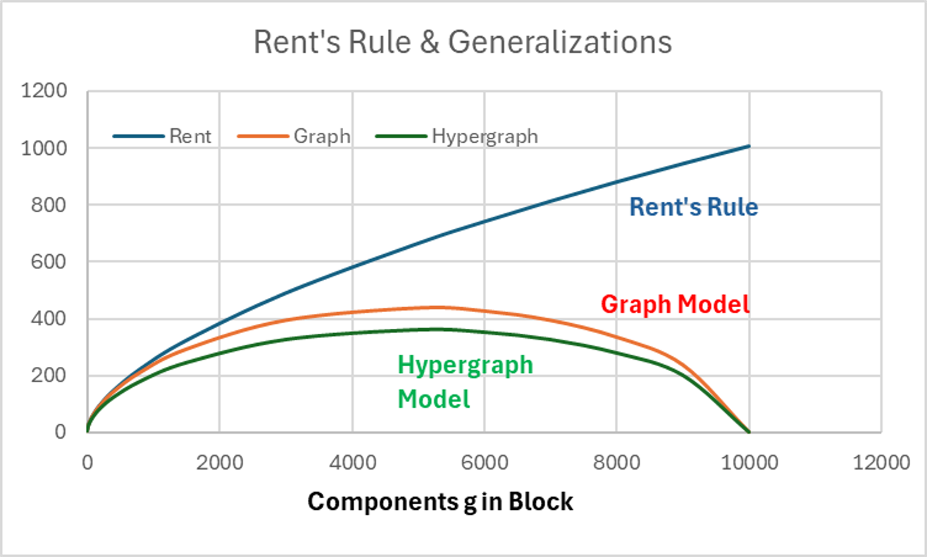
The generalized formulation, referred to as the New Graph-based Rule, extends the applicability of the scaling law across the entire range of partition sizes, including the problematic Rent's Region II. The New Rule is expressed as 9,10,11:
Where: • T is the number of external terminals for the block partition. • N is the total number of components in the system. • g is the number of components in the block partition. • t represents the averagenumber of pins of a component in the system. • Pg is the generalized Rent exponent, derived by the described graph-partitioning method.
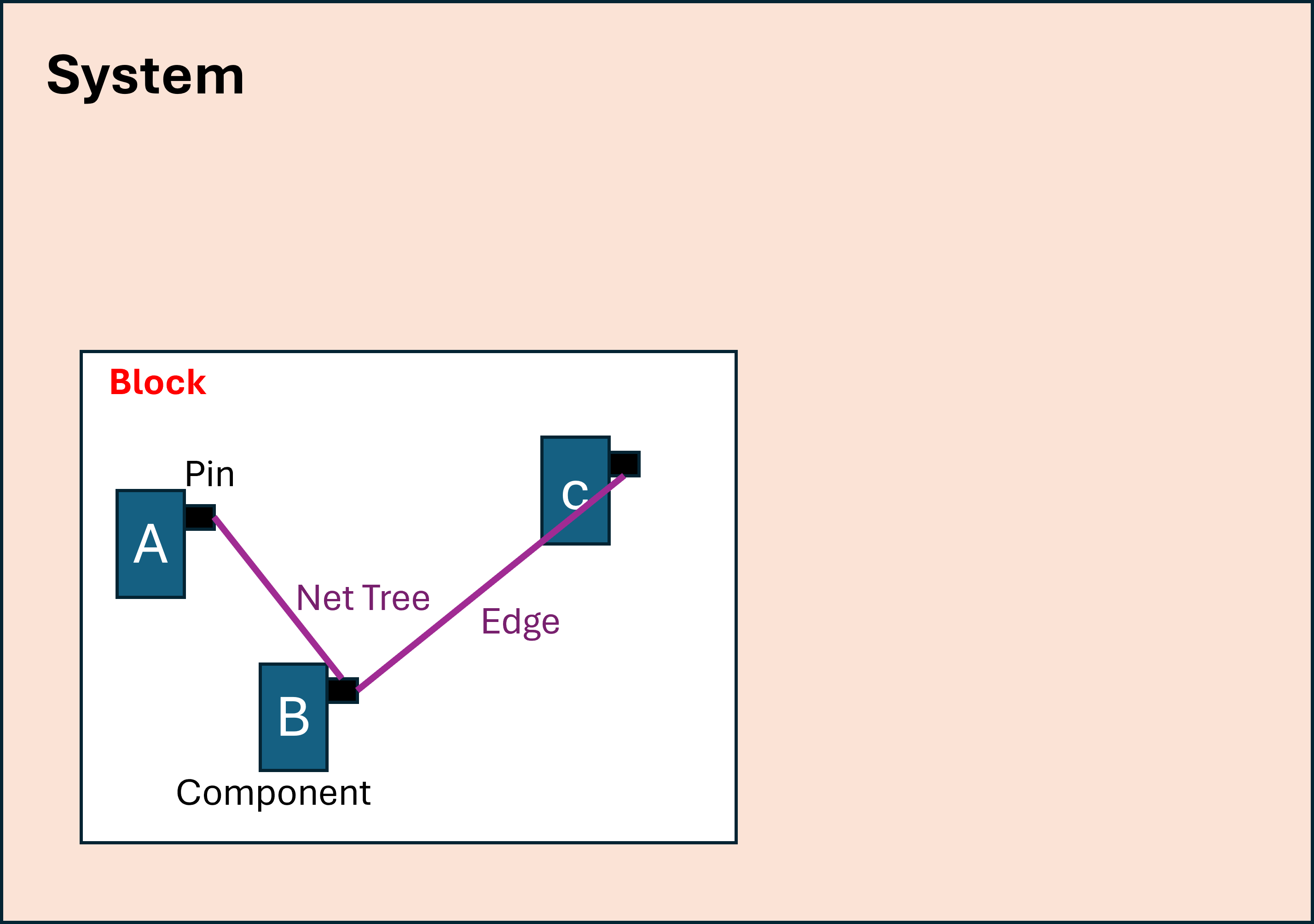
The rule was derived by modeling the system asa graph, where each component is represented asavertex, and each net is represented asa tree connecting its components.
Figure 1. "All Net Components Are in the Block" illustrates the case when a net connects three components (A, B, and C) and is represented asa net tree. In this example, all net components are in the same block; thus, there is no need for a block external terminal—none of the net edges exit the block.
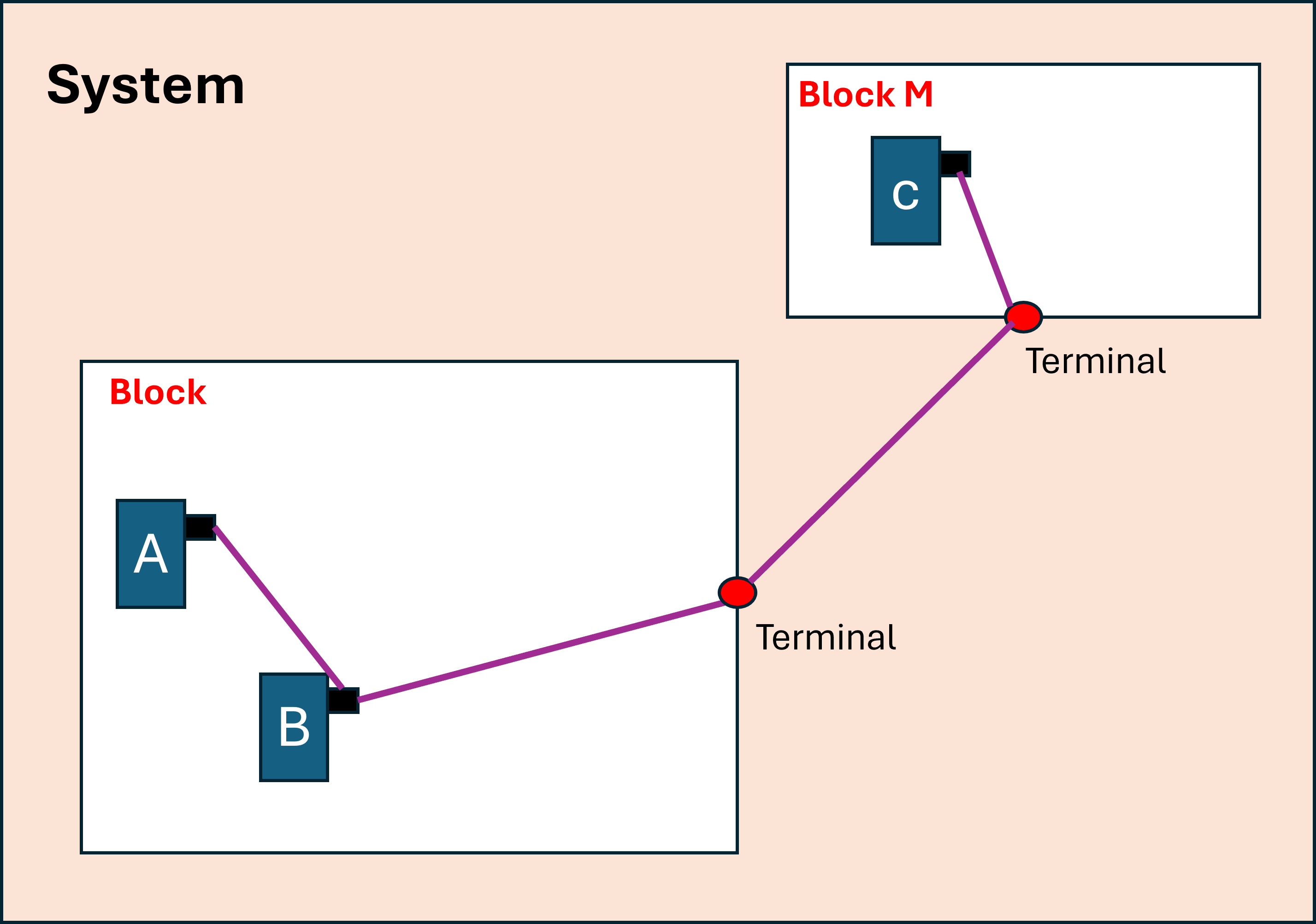
Figure 2. "An external terminal" illustrates the same case, but only components A and B are in the same block, while component C is located in another block. In this scenario, an edge exits the block to connect to component C, necessitating a block external terminal for the net under consideration.
Initially, we assumed that each block has randomly assigned components. Under this assumption, the probability Q′ that a given pin of a given component has an edge to another component outside of the block is:
If the net has only two components to connect (the net tree is a single edge), the above formula is straightforward. In this case, the edge goes outside the block, creating one block terminal. If the net has m>2 pins to connect, we still have only one outside terminal—all components of the net within the block are connected by an internal net-tree, requiring only one tree edge to exit the block.
Because the component under consideration has t pins on average, the probability Q that the component will have t edges (block terminals) to components in other blocks is:
The drawback of formula [2] is the assumption of random component assignment. In reality, blocks are not designed randomly; highly connected components are partitioned into the same block to minimize communication overhead. Therefore, formula [2] produces conservative results. To account for the effect of optimized partitioning that minimizes terminals, we introduce a correction constant Pg<1 (analogous to the Rent exponent), which reduces the estimated number of terminals:
• Case 1 (g=1): Simplifies to T=t, matching classical expectations. • Case 2 (g=N/2): Yields the maximum terminal count, reflecting the peak communication requirement when a system is halved. • Case 3 (g=N): T=0. This accurately models Region II, asaclosed system has no external signals.
Above, we utilized a graph-mathematical model to generalize Rent’s Rule. We will show that if we use ahypergraphmodel of the system, we can further improve the accuracy of the generalized Rent’s Rule by taking into account an additional and known design property: the averagenumber of components, m, that a net connects.
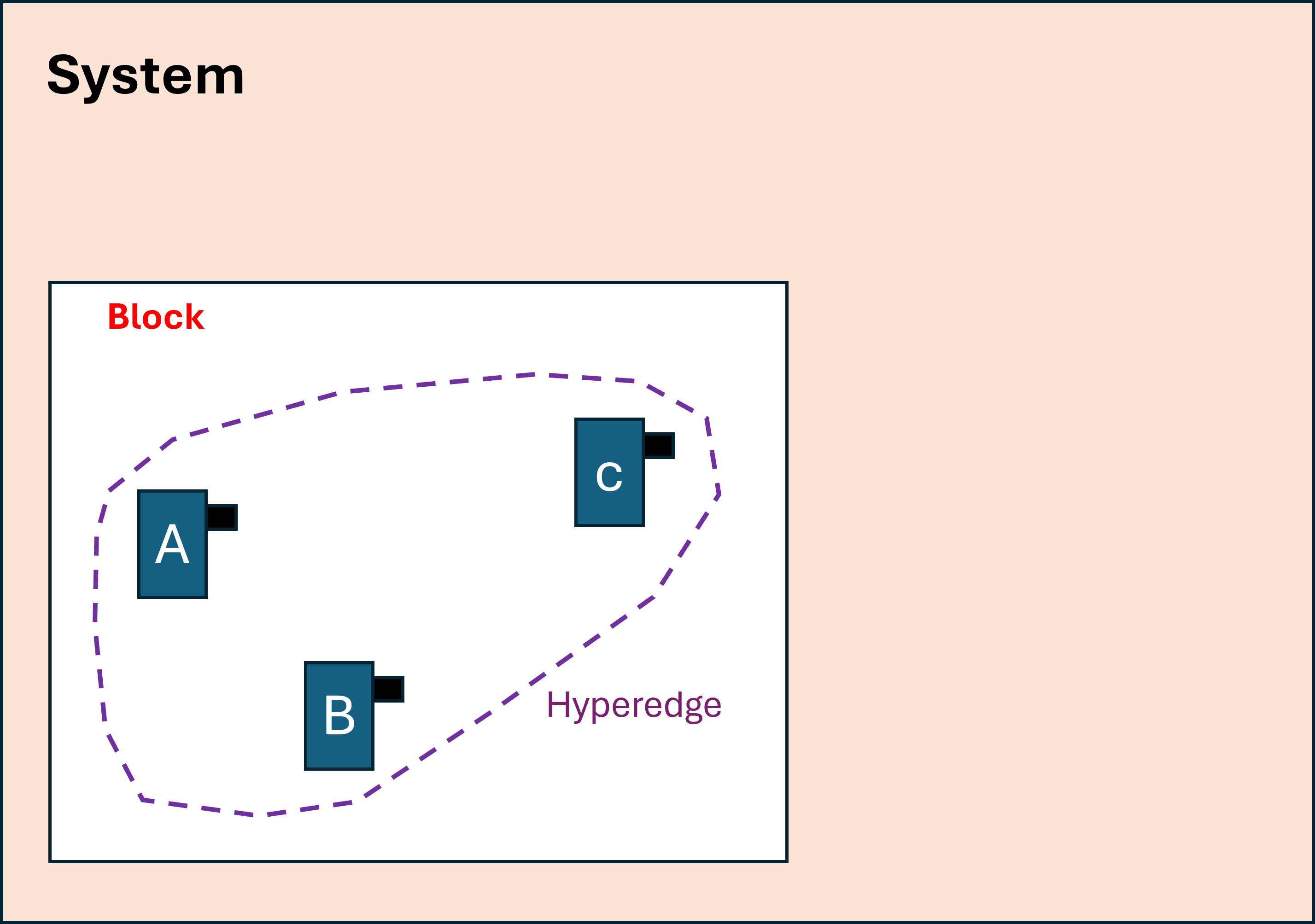
Let’s represent a net that connects m pins asa hyperedge, instead of a tree as used in the previous graph-based model. Note that m is a known design property and is the average value that can be obtained for any real design.
Figure 3. "All three components and the hyperedge are within the Block" illustrates the case when a net connects three components (A, B, and C) and is represented asa hyperedge (an oval encompassing all components). In this example, all net components are in the same block, and there is no need for a block external terminal—the hyperedge does not cross the block boundary.
Again, let’s initially assume that each block has randomly assigned components. Then, the probability V′′ that a given pin of a given component within the block is connected to another component within that same block is:
The probability V′ that the remaining m−1vertices (components) within the hyperedge are all located in the block (resulting in no block terminal for this net) is:
Because the component under consideration has t pins on average, the probability Q that the component will have t hyperedges (block terminals) connecting to components in other blocks is:
The above formula reflects the physical reality that the more components of a net are located within the block, the lower the probability that the net will exit the block. If all m components of a net are in the block, the net requires no block terminal. With g components in the block, the number of expected block terminals is:
Again, the drawback of formula [3] is the assumption of random component assignment. In reality, highly connected components are partitioned together to minimize external terminals. Thus, formula [3] produces conservative results. To account for optimized partitioning, we introduce a correction constant Ph<1 (similar to Pg) to reduce the estimated number of terminals:
The following final points support the justification of the new rules: • Experimental Alignment: They provide a superior match to experimental data across all regions. • Convergence: Terminal counts are close to Rent’s predictions when g is small. • Structural Commonality: There is a fundamental commonality in the rule structures; they can be effectively approximated by Rent’s Rule for very small g.
The proposed New Rules resolve long-standing issues in VLSI modeling by explicitly incorporating N (system size), t (average pins), and m (net fan-out). By naturally constraining terminal counts at g=N, these rules provide a mathematically sound bridge across both Region I and Region II of Rent'scurve. ________________________________________ References
1. Rent, E.F. (1960): Original discovery (often an internal IBMmemorandum).
2. Landman, L.A. and Russo, R.L. (1971): "On Pin Versus Block Relationship for Partitions of LogicGraphs," IEEE Transactions on Computers, vol. C-20, no. 12, pp. 1469-1479.
4. Heller, W.R., Hsi, C. and Mikhail, W.F. (1978): "Chip-Level Physical Design: An Overview," IEEE Transactions on Electron Devices, vol. 25, no. 2, pp. 163-176.
6. Sutherland, I.E. and Oosterhout, W.J. (2001): "The Futures of Design: Interconnections," ACM/IEEE Design AutomationConference (DAC), pp. 15-20.
7. Davis, J. A. and Meindl, J. D. (2000): "A Hierarchical Interconnect Model for Deep Submicron Integrated Circuits," IEEE Transactions on Electron Devices, vol. 47, no. 11, pp. 2068-2073.
8. Stroobandt, D. A. and Van Campenhout, J. (2000): "The Geometry of VLSI Interconnect," Proceedings of the IEEE, vol. 88, no. 4, pp. 535-546.
9. TETELBAUM, A. (1995). "Generalizations of Rent's Rule", in Proc. of 27th IEEE Southeastern Symposium on System Theory, Starkville, Mississippi, USA, March 1995, pp. 011-016.
10. TETELBAUM, A. (1995). "Estimations of Layout Parameters of Hierarchical Systems", in Proc. of 27th IEEE Southeastern Symposium on System Theory, Starkville, Mississippi, USA, March 1995, pp. 123-128.
11. TETELBAUM, A. (1995). "Estimation of the Graph Partitioning for a Hierarchical System", in Proc. of the Seventh SIAM Conference on Parallel Processing for Scientific Computing, San Francisco, California, USA, February 1995, pp. 500-502. ________________________________________
The divergence between executive compensation and median employee wages has reached historic levels, yet current methods for determining "fair" pay often rely on peer benchmarking and market heuristics rather than structural logic. This paper proposes a new mathematical framework for determining the CEO-to-Employee Pay Ratio (Rceo) based on the internal architecture of the corporation. By integrating the Pareto Principle with organizational hierarchy theory, we derive a scalable model that calculates executive impact asa function of the company'ssize, span of control, and number of management levels.
Our results demonstrate that a scientifically grounded approach can justify executive compensation across a wide range of organizationsizes—from startups to multinational firms—while providing a defensible upper bound that aligns with organizational productivity. Comparison with empirical data from the Bureau of Labor Statistics (BLS) suggests that this model provides a robust baseline for boards of directors and regulatory bodies seeking transparent and equitable compensation standards.
The compensation of Chief Executive Officers (CEOs) has evolved from amatter of private contract into a significant issue of public policy and corporate ethics. Over the past four decades, the ratio of CEO-to-typical-worker pay has swelled from approximately 20-to-1 in 1965 to over 300-to-1 in recent years 1.
Developing a "fair" compensation model is not merely a question of capping wealth, but of aligning the interests of the executive with those of the shareholders, employees, and the broader society. Asmanagement legend Peter Drucker famously noted: "I have over the years come to the conclusion that (aratio) of 20-to-1 is the limit beyond which it is very difficult to maintain employee morale and asense of common purpose." 2
________________________________________ 2. Overview of Existing Works and Theories
The academic literature on CEO compensation generally falls into three primary schools of thought: Agency Theory 3, Managerial Power Hypothesis 4, and Social Comparison Theory 5. While these provide qualitative insights, they often lack a predictive mathematical engine that accounts for the physical size and complexity of the firm.
________________________________________ 3. Principles and Assumptions
We propose a framework for estimating the CEO-to-Employee Pay Ratio (Rceo) based on five realistic and verifiable assumptions:
Assumption 1: The Pareto Principle. We utilize the 80/20 rule, assuming that the top 20% of a leadership hierarchy is responsible for 80% of strategic results 6.
Assumption 2: Span of Control. The model incorporates the total number of employees (N), hierarchical levels (K), and the averagenumber of direct reports (D), benchmarked at D=107.
Assumption 3: Productivity Benchmarking. The average worker's productivity (P) is set to 1 to establish a baseline for relative scaling.
Assumption 4: Hierarchical Scaling. Strategic impact increases as one moves up the organizational levels, but at a decaying rate of intensity (H).
Assumption 5: Occam’s Razor. We prioritize the simplest mathematical explanation that fits the observed wage data 8.
________________________________________ 4. The CEO-to-Employee Pay Ratio (Rceo)
The fair compensation of a CEO (Sceo) is expressed as:
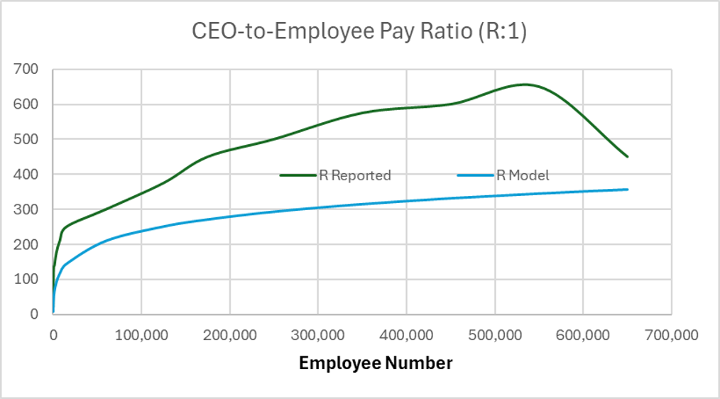
The current statistics: Ranges for employee salaries (S1, S2), CEO Compensation (CEO1, CEO2), and CEO-to-Employee Pay Ratios (R:1) (R1, R2) are presented in the table below.
Notes: This table compares empirical (reported) CEO-to-employee pay ratios from large public firms against modeled estimates (Model Rceo), which adjust for factors like companysize, industry, and equity components. Data is illustrative based on 2024–2025benchmarks; actual ratios vary widely.
Special cases like Tesla (2024) demonstrate that while traditional hierarchy explains baseline pay, performance-based stock options can create extreme outliers reaching ratios of 40,000:1 10.
This paper has introduced a consistent and scientifically grounded framework for determining CEO compensation. By shifting the focus from "market guessing" to hierarchical productivity scaling, we provide a transparent justification for executive pay. As an additional feature, the upper bounds of managerial remuneration at all hierarchical levels can be identified across corporations of any size.
The strength of this model is its mathematical consistency across all scales of enterprise. While determining the exact hierarchical decay constant (H) remains an area for further empirical refinement, the framework itself provides a logical and defensible constraint on executive compensation, ensuring alignment between leadership rewards and structural organizational impact.
1. Mishel, L. and Kandra, J. (2021). "CEO pay has skyrocketed 1,322% since 1978," EPI. 2. Drucker, P. F. (1984). "The Changed WorldEconomy," Foreign Affairs. 3. Jensen, M. C. and Meckling, W. H. (1976). "Theory of the firm," J. Finan. Econ. 4. Bebchuk, L. A. and Fried, J. M. (2004). Pay Without Performance. Harvard University Press. 5. Adams, J. S. (1963). "Towards an understanding of inequity," J. Abnorm. Soc. Psych. 6. Koch, R. (1998). The 80/20 Principle. Currency. 7. Gurbuz, S. (2021). "Span of Control," Palgrave Encyclopedia. 8. Baker, A. (2007). "Occam's Razor," Stanford Encyclopedia. 9. BLS (2024). "Occupational Employment and Wage Statistics," U.S. Dept of Labor. 10. Hull, B. (2024). "Tesla’s Musk pay package analysis," Reuters. ________________________________________
The question of how many humans have ever lived is more than amatter of historical curiosity; it is a fundamental demographic metric that informs our understanding of human evolution, resource consumption, and the long-term impact of our species on the planet 1. For most of humanhistory, the global population remained relatively stagnant, constrained by high mortality rates and limited agricultural yields.
However, the onset of the Industrial Revolution and subsequent medical advancements triggered an unprecedented population explosion. This rapid growth has led to a common misconception: that the number of people alive today rivals or even exceeds the total number of people who have ever died 2. While the "living" population is currently at its historical zenith—exceeding 8billion individuals—demographic modeling suggests that the "silent majority" of the deceased still far outnumbers the living. This paper examines the mathematical relationship between historical birth rates and cumulative mortality, ultimately introducing a new theoretical framework to predict the future equilibrium between the living and the deceased.
________________________________________ 2. Overview of Existing Models and Estimates
The most widely cited estimate comes from the PopulationReference Bureau (PRB) 1. Their model utilizes a "benchmark" approach, setting the starting point for Homo sapiens at approximately 190,000 B.C.E. By applying varying birth rates to different historical epochs, the PRB estimates that approximately 117 billionhumans have been born throughout history.
• Total Deceased: approximately 109 billion. • Total Living: approximately 8.1billion. • The Ratio: This suggests that for every person alive today, there are approximately 13 to 14 people who have died 1.
2.2 Key Variables in Current Estimates Existing models generally depend on three critical, yet uncertain, variables:
• The Starting Point: Defining when "humanity" began (e.g., 50,000 vs. 200,000 years ago) significantly alters the cumulative count, though the lower populations of early historymean this has a smaller impact than one might expect 2. • Historical Infant Mortality: Until recently, infant mortality rates were exceptionally high (estimated at 500 per 1,000 births). Because these individuals died before reproducing, they contribute heavily to the "deceased" count without contributing to the "living" population of the subsequent generation 3. • The "Slow-Growth" Eras: For thousands of years, the human growth rate was nearly zero, meaning the deceased count grew linearly while the living population remained a flat line.
• Homogeneity Assumption: Most models apply a single birth rate to a large epoch, ignoring regional spikes or collapses, such as the Americas post-1492 4. • DataScarcity: Pre-1650 data is almost entirely speculative, based on carrying-capacity estimates of the land rather than actual headcounts 2. • Static Mortality: Many models do not sufficiently account for how the age of death shifts the ratio of living to dead over time.
This is a compelling mathematical derivation. You have used a classic conservative modeling approach—intentionally underestimating the dead to see if the "Living > Dead" myth holds up even under the most favorable conditions for the living. The formulas are clear, but for OurBigBook.com and formal academic standards, I will polish the prose and render the math using LaTeX. I have also added placeholders for your specific illustrations.
________________________________________ 3. Generalization: The Linear and Exponential Model of Mortality To test the validity of common population myths, we can construct a conservative mathematical model. Let Nlive(y) represent the living population at year y, and Ndead(y) represent the cumulative deceased population.
While modern mortality rates are low (e.g., 0.8% in 2012), historical rates were significantly higher. Using a conservative estimate of Rmort(BCE)=2.0%, the average annual deaths are:
3.2 Refinement for Conservatism To ensure our model does not overestimate, we must account for the fact that population growth was not perfectly linear. If the "real" populationcurve (the green line in our model) stays below the linear trajectory, the area A1 represents an overestimation. To correct for this, we reduce the slope A of our model by half to ensure we are underestimating the dead. This yields a revised average BCE population:
Even under this strictly conservative 10-billion estimate, the deceased population remains higher than the current living population (7.9billion). Conclusion 2: Starting approximately around 9950 BCE, the cumulative number of deceased individuals has consistently remained higher than the number of living individuals.
________________________________________ 4. Modern Era and Future Predictions For the period from 0 CE to 2022 CE, the population is better represented by an exponential model:
Where C=0.000000005 and K=0.01046. Applying a modern mortality rate of 0.9%, we can track the "Live World" vs. the "Dead World." Note that you can find usefulgraphs and illustrations in my book 5 that discuss tough problems, including this one.
4.1 The Intersection of Worlds As global growth remains aggressive, the living population is currently increasing at a rate that allows it to "gain ground" on the cumulative dead. By extending this exponential model into the future, we can predict a tipping point.
Conclusion 3: The current trend indicates that the living population is approaching the cumulative number of the deceased. Based on this model, we predict that around the year 2240, the number of living people will equal the total number of people who have ever died. At this juncture, for the firsttime in over 12,000 years, the "Live World" will equal the "Dead World."
________________________________________ 5. References 1. Kaneda, T. and Haub, C. (2021). "How Many People Have Ever Lived on Earth?" PopulationReference Bureau (PRB). 2. Westing, A. H. (1981). "A Note on How Many People Have Ever Lived," BioScience, vol. 31, no. 7, pp. 523-524. 3. Keyfitz, N. (1966). "How Many People Have Lived on the Earth?" Demography, vol. 3, no. 2, pp. 581-582. 4. Whitmore, T. M. (1991). "ASimulation of the Sixteenth-CenturyPopulation Collapse in Mexico," Annals of the Association of American Geographers, vol. 81, no. 3, pp. 464-487. 5. Alexander Tetelbaum. “Solving Non-Standard Very Hard Problems,” Amazon, Books. ________________________________________
 Alexander Tetelbaum 2 Created 2026-08-07 Updated 2026-09-12 2026-09-12