An isolated singularity at $a$ means that the function is holomorphic throughout some punctured disc $0<|z-a|<r$. Its residue is the Laurent coefficient $c_{-1}$, equivalently $(2\pi i{)}^{-1}{\int }_{|z-a|=\rho }f(z)dz$. The singularity is removable if all negative Laurent coefficients vanish, a pole of order $k$ if only finitely many are nonzero and the lowest power is $-k$, and essential if infinitely many negative coefficients are nonzero.

For the final contour integral, expand $e^{tz}{e}^{t/z}$. On the circle these exponential series converge absolutely and uniformly for $t$ in every bounded set, so their product can be integrated term by term. Inonly $j-k-2=-1$ contributes. Set $k=m$, $j=m+1$. ThusThe resulting power series converges for every complex $t$ by the ratio test. The coefficients are independent of the positive radius $R$.

For the polynomial ring, use the Euclidean function $\delta (f)=\mathrm{deg}f$ on nonzero polynomials. If $a,b\in F[X]$ and $b\ne 0$, subtract the multiple of $b$ that cancels the leading term of $a$. The leading coefficient of $b$ is invertible in the field, and every subtraction strictly lowers the degree of the remainder. This process terminates with $a=qb+r$ and either $r=0$ or $\mathrm{deg}r<\mathrm{deg}b$. Thus $\boxed{F[X]\text{ is a Euclidean domain}}$.

For the Gauss lemma for polynomials, call an integer polynomial primitive when its coefficient gcd is one. If two primitive polynomials had a nonprimitive product, a prime $p$ would divide every product coefficient. Reducing modulo $p$ would give a zero product of two nonzero polynomials in the integral domain ${\mathbb{F}}_p[X]$, a contradiction. Therefore the product of primitive integer polynomials is primitive.

To transfer a rational factorization, write each nonzero rational factor as a rational scalar times a primitive integer polynomial by clearing denominators and removing the coefficient gcd. Thus $f=qAB$ with primitive $A,B\in \mathbb{Z}[X]$ and $q\in \mathbb{Q}$. Their product is primitive by the lemma. If $q=m/n$ in lowest terms, integrality of every coefficient of $f$ forces $n$ to divide every coefficient of $AB$, so $n=1$. Hence $q\in \mathbb{Z}$; absorbing $q$ into either factor produces the required integer factorization with the same positive factor degrees. In particular irreducibility of a primitive polynomial over $\mathbb{Z}$ and over $\mathbb{Q}$ is equivalent.

Finally, let $a/b$ in lowest terms, $b>0$, be a rational root of a monic degree-$d$ integer polynomial. Multiplying the equation by $b^d$ shows $b\mid a^d$. Coprimality forces $b=1$. Thus $\boxed{\text{every rational root of a monic integer polynomial is an integer}}$.

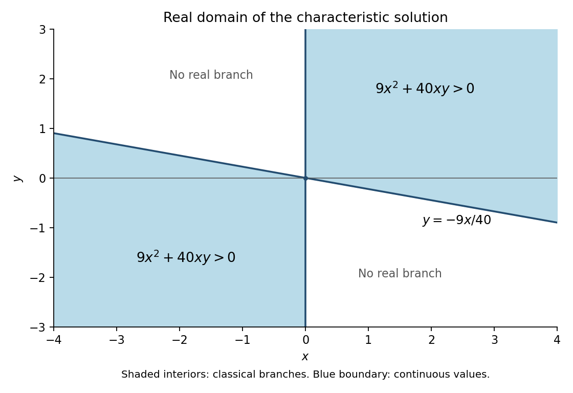
Use the characteristic parameter $t$ and writeDirect differentiation givesA characteristic beginning at $(s,0,0)$ therefore satisfies $5x+4y+3u=5s$ and $x^2+y^2+u^2=s^2$. Eliminating $s$ givesIts discriminant as a quadratic in $u$ is $100(9x^2+40xy)$. Requiring the root to be zero when $y=0$ selectsThe selected branch is differentiable in each of the two regions where the radical is strictly positive, and substitution into the differentiated quadratic identity verifies the partial differential equation there. On the initial line away from the origin the characteristic vector has nonzero $y$ component $-3s$, so these are the locally unique branches determined by that line.

The maximal real-valued continuation of these branches has the printed domainAt $x=0$ the continuous limiting value is $u(0,y)=3y/4$. The two bounding lines are $x=0$ and $y=-9x/40$, and the included sectors are the one above the sloping line on the right and the one below it on the left.

As in the fold boundary of a characteristic graph, the closed-domain statement concerns the formula's real values. A classical solution requires first derivatives on an open set. Along the nonzero boundary points $9x^2+40xy=0$, the radical's transverse derivative is singular, so the formula is generally not a classical solution there; its two classical domains are the interiors of the shaded sectors. The origin is characteristic for the initial data and does not supply a differentiable neighborhood solution. This qualification preserves the source's stated closed set while distinguishing it from the domain of a classical solution.

Differentiate the Wronskian:It is therefore constant. Linear dependence plainly makes it zero. Conversely, if it is zero, the two initial-data vectors $(u(0),u^{\prime }(0))$ and $(v(0),v^{\prime }(0))$ are linearly dependent. Some constants $A,B$, not both zero, make $Au+Bv$ and its derivative zero at zero. Uniqueness for a linear second-order equation with continuous coefficients then makes $Au+Bv$ identically zero. Thus $\boxed{w=0⟺u,v\text{ are linearly dependent}}$.

For the prescribed integral put $K(x,s)=[u(x)v(s)-u(s)v(x)]/w$. Then $K(x,x)=0$, $K_x(x,x)=-1$, and $K_{xx}(x,s)=-q(x)K(x,s)$. Differentiation under the integral, using continuity of the coefficients and forcing, givesThis proves the required inhomogeneous equation, with the sign of the forcing as printed.

For the explicit forcing take $u=\cosh x$, $v=\sinh x$, so $w=1$ and $K(x,s)=-\sinh (x-s)$. Since $2/(e^s+e^{-s})=\mathrm{sech}s$, the integral isIndeed expand $\sinh (x-s)=\sinh x\cosh s-\cosh x\sinh s$ and integrate $1$ and $\tanh s$. Adding the entire homogeneous solution givesFinally multiply the other equation by $\sin x$ and integrate from zero to $\pi$. Integration by parts givesThus $\boxed{{\int }_0^{\pi }f(s)\sin sds=0}$ is necessary. It is also sufficient: the solution with $y(0)=0$ is $B\sin x-{\int }_0^x\sin (x-s)f(s)ds$, and the integral condition gives its value zero at $\pi$.