Draw a failure envelope in the $({\sigma }_n^{\prime },\tau )$ plane. A useful brittle shear-failure approximation is the Mohr-Coulomb failure criterionwhere $c$ is cohesion, $\phi$ the internal friction angle, and ${\sigma }_n^{\prime }$ the effective compressive normal stress. A circle wholly inside the envelope is below this ideal failure threshold. Increasing the differential stress expands it until it first touches the envelope: the tangent points identify the failing plane orientations. For a linear envelope, tangency impliesWith the angle convention above, the upper tangent point is at $2\theta =90^{\circ }+\phi$. Its plane therefore makes $45^{\circ }-\phi /2$ with the maximum-compression direction; there is a conjugate plane on the other side. For $\phi =30^{\circ }$, this is $30^{\circ }$, rather than the $45^{\circ }$ plane of maximum shear stress. An existing weak fault can reactivate first, with its own lower cohesion and friction, and need not have this optimum new-fracture orientation.

For tensile brittle fracture, add a tensile strength cutoff: failure occurs when ${\sigma }_3^{\prime }\le -T_0$, where $T_0>0$. The opening fracture is approximately perpendicular to the minimum-compression direction. Real rock envelopes curve, especially at small confinement; a straight shear envelope must not be extrapolated as an exact tensile law. High confinement can instead favor distributed or ductile deformation, so merely drawing a larger circle does not establish that brittle failure is the active mechanism.^[ref]

For a plane whose normal lies in the ${\sigma }_1$–${\sigma }_3$ plane, rotate through $2\theta$ from $({\sigma }_1,0)$ in the stated sign convention. The circle point givesThe normal-to-plane angle is essential: if the angle supplied is between the plane itself and ${\sigma }_1$, use its complement for $\theta$. The principal stress planes have zero shear stress, and planes at $45^{\circ }$ to those principal stress planes have maximum $|\tau |$.

For an arbitrary plane in a fully three-dimensional stress field, let $n_i$ be its direction cosines in the principal stress basis. ThenThese follow by resolving the traction into its normal and tangential components; the compression-positive tensor is the negative of the usual tension-positive Cauchy stress tensor. The family of Mohr circles visualizes the possible combinations, but the two-dimensional $2\theta$ rule alone does not specify an arbitrary three-dimensional orientation.^[ref]

Near the south magnetic pole, the inducing magnetic field and induced magnetic moment are vertically upward. Directly over the car its dipole field is also upward, again reinforcing the main field. The total-field magnetic anomaly is therefore the same positive central high and weak negative side lobes as at the north magnetic pole under the same induced-dipole assumptions. A fixed signed vertical field component would reverse, but the scalar field strength measured by the proton-precession magnetometer does not. If the car's remanent magnetization dominates, neither this symmetry nor these predicted signs is assured.

At the magnetic equator, the inducing magnetic field and induced magnetic moment are horizontal. Let $x$ point along this field, approximately magnetic north, and $y$ across it. Directly over the car, the dipole field opposes the main field, producing a negative central total-field magnetic anomaly. A north–south traverse through the car givesa symmetric central low with positive shoulders. An east–west traverse through the car instead has $\Delta T(y)\propto -(y^2+h^2{)}^{-3/2}$, a single negative trough. The equatorial anomaly therefore needs a stated traverse orientation; there is no universal single equatorial line profile.

Near the north magnetic pole, take the inducing magnetic field and induced magnetic moment as vertically downward. Directly above the car, its anomalous field reinforces the main field: a positive central total-field magnetic anomaly results. Along a horizontal traverse, the vertical-dipole approximation gives a symmetric central high flanked by weaker negative side lobes:where $h$ is the depth from the sensor to the effective dipole centre. The anomaly width scales with $h$; no absolute amplitude can be calculated without the car's magnetic moment.

For the fully gas-filled reservoir,soBoth impedances are now smaller than those of the cap rock. Both reflections reverse seismic reflection polarity, with a substantially larger amplitude for the P wave reflection. Reading the right-hand $V_p$ endpoint instead as $1.20\mathrm{km}{\mathrm{s}}^{-1}$ would give $R_p\simeq -0.20$, preserving the interpretation.

For the fully water-filled reservoir, the approximate densities and wave speeds giveand henceBoth are positive: the reservoir has larger P wave and shear-wave impedances than the cap rock, and neither reflection reverses the chosen stress-wave seismic reflection polarity.

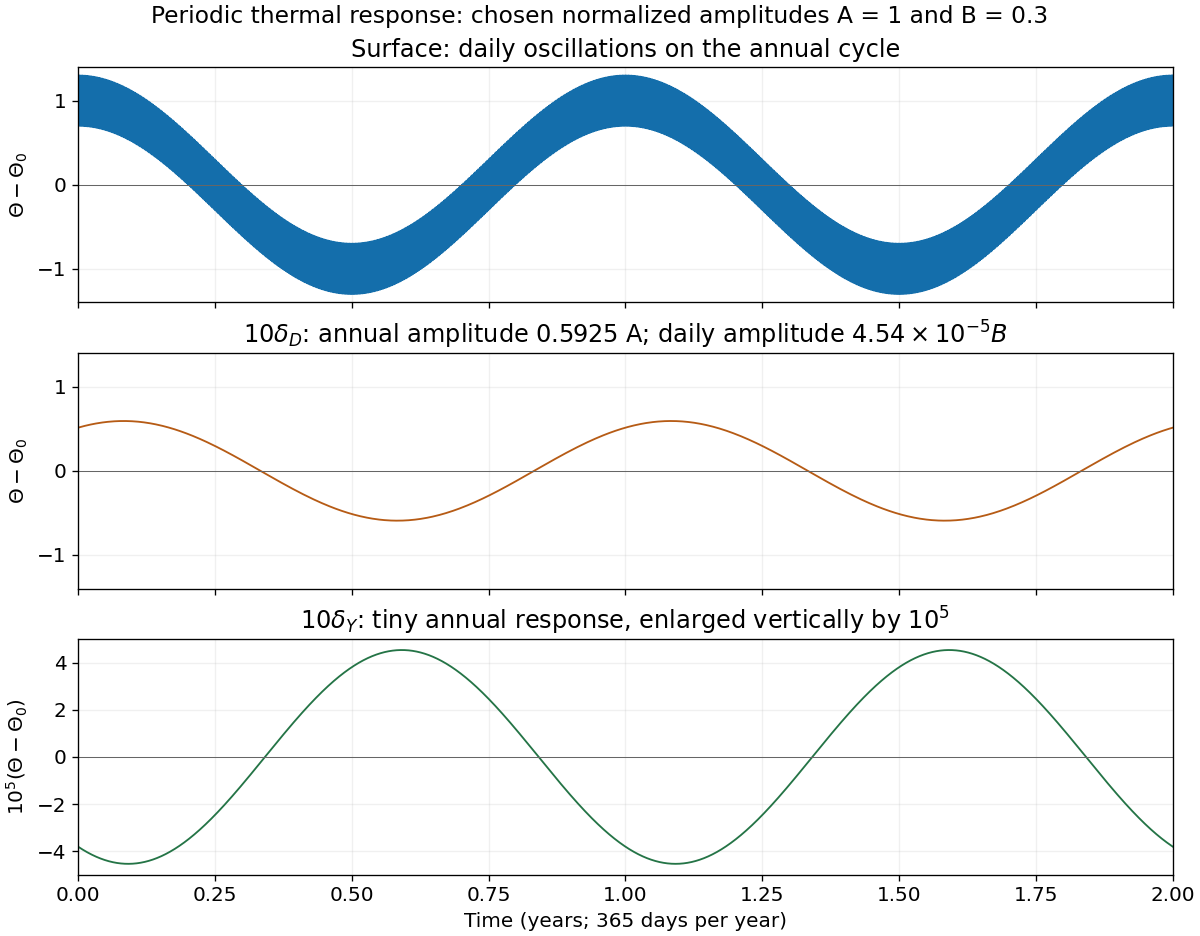
At $x=10{\delta }_Y$, the annual attenuation is $e^{-10}$ and the daily attenuation is $e^{-10\sqrt{365}}$, approximately $10^{-83}$. ThusOn the same vertical scale as the surface plot this is almost the constant ${\Theta }_0$. With a sufficiently enlarged scale, a residual annual oscillation of amplitude $4.54\times 10^{-5}A$ remains. Its phase lag is ten radians, interpreted modulo $2\pi$ when comparing periodic maxima.

At $x=10{\delta }_D$, the daily component is multiplied by $e^{-10}\simeq 4.54\times 10^{-5}$ and has a lag of ten radians. The annual component instead has $x/{\delta }_Y=10/\sqrt{365}\simeq 0.5234$. HenceThe sketch is nearly a smooth annual sinusoid, with annual amplitude about $0.5925A$ and annual phase lag about $0.5234$ radians, corresponding to about $30.4$ days on the chosen year scale. The tiny daily component is retained in the formula rather than declared identically zero.

At the surface both attenuation factors are one and both lags vanish:The sketch is a rapid daily oscillation on a slowly varying annual background. The amplitudes cannot be inferred uniquely from the sampling intervals alone.

The adequately sampled record shows a yearly cycle and a daily cycle. Up to exchanging their labels,Using $365$ days per year for numerical estimates,These are angular frequencies. The corresponding ordinary frequencies are $1\mathrm{y}{\mathrm{r}}^{-1}$ and $1\mathrm{da}{\mathrm{y}}^{-1}$.

The source text and its figure are inconsistent here. The plotted low-frequency maximum in W is near $0.0055\mathrm{da}{\mathrm{y}}^{-1}$, rather than the printed $0.055\mathrm{da}{\mathrm{y}}^{-1}$. The original PDF shows that this discrepancy is already present in the examination, rather than introduced by transcription.

Machine 2 records only about half a year. Its first nonzero discrete Fourier transform bin is therefore atThe annual component near $1/365\mathrm{da}{\mathrm{y}}^{-1}$ is below that first bin. The finite window function spreads it through spectral leakage, with a prominent first-bin contribution. This explains the plotted peak without invoking a new physical period.

A literal peak at $0.055\mathrm{da}{\mathrm{y}}^{-1}$ would instead have a period of about $18.2$ days. Neither the two stated model frequencies nor the given sampling schedule identifies such a separate component. The interpretation above treats the printed decimal as an apparent typo; it does not silently change the stated number.

The true daily component has $f_D=1\mathrm{da}{\mathrm{y}}^{-1}$, above machine 3's Nyquist frequency. At sampling times $t_n=2n/3$ days,The last sequence is also produced by a continuous cosine with frequency $0.5\mathrm{da}{\mathrm{y}}^{-1}$ sampled at those same times. Hence the observed peak is the sampled sinusoid aliasIt is not evidence for an additional two-day physical temperature cycle.

The conventional Nyquist frequency isFrequencies above this cutoff are indistinguishable from lower-frequency sampled sinusoid aliases. The Nyquist–Shannon sampling theorem requires a band limit strictly below the cutoff for general phase information: at exactly the cutoff, some phases can give zero samples. Thus $32$ hours is the conventional limiting period, with unambiguous reconstruction requiring a longer period under those sampling assumptions.

Sixteen hours is $2/3$ of a day, so the sampling rate is

The consistent matching is:

Series C stops after about six months, identifying machine 2. Its short record gives spectrum W a coarser Fourier frequency resolution. Series A resolves the annual variation but misses the changing daily phase: the regular three-day interval samples the daily oscillation at the same phase, so its daily contribution aliases to a constant. Its spectrum is Y. Machine 3 produces the half-daily-frequency alias in X, leaving D as its time series. The fully sampled two-year record B and spectrum Z agree with the supplied first row.

These identifications use the record lengths, frequency locations and sampling intervals. They do not require assuming that the plotted spectral heights have an identical normalization.

The amplitude relative to the zero mean is $1\mathrm{V}$. The peak-to-peak excursion is $2\mathrm{V}$.

The angular frequency is $\omega =2\pi /T=\pi /2\mathrm{rad}{\mathrm{s}}^{-1}$. This is distinct from the ordinary frequency in cycles per second.

The ordinary frequency is $\nu =1/T=0.25\mathrm{Hz}$, or one quarter of a cycle per second.

The waveform repeats after one positive and one negative interval, so its fundamental period is $T=4\mathrm{s}$. A two-second shift reverses its sign and is not a period.