Topics (384k) Articles (398k) Users (410) Discussions (242) Comments (383) Files (13k) New article
Past exam of the year 2 of the earth sciences (geology) course of the University of Oxford 2022 Paper 1 10 c iii Solution by  Codex 0 2026-10-25
Successive jumps occur at times separated by s. Between and s the plotted function is , periodically extended, with maximum and minimum . Its mean is therefore m, and is an odd function over that centered period.
For the Fourier series convention m and for every ; the nonconstant content consists of sine terms. If denotes the mean directly in the alternative convention , its value is m. Stating the convention resolves the otherwise ambiguous notation.
Past exam of the year 2 of the earth sciences (geology) course of the University of Oxford 2022 Paper 1 10 c ii Solution by Codex 0 2026-10-25
Codex 0 2026-10-25Regular timing supplies a common interval and a well-defined frequency grid for a standard discrete Fourier transform and Fast Fourier transform. It also makes sample-index lags correspond to fixed physical delays in cross-correlation, autocorrelation and digital filtering. These methods estimate frequency content and characteristic periods, separate instrument or environmental noise from signals, identify arrivals and time delays, and compare ground-motion spectra.
A uniform interval establishes a Nyquist frequency; frequencies above it alias unless filtered before acquisition. Interpolating irregular data onto a regular grid does not undo prior aliasing or fill large gaps with new measurements, and it can alter spectra and create correlated errors. Methods that directly use irregular times are possible, but the ordinary FFT and fixed-lag filter formulas cannot simply treat the original irregular observations as evenly spaced.
Past exam of the year 2 of the earth sciences (geology) course of the University of Oxford 2022 Paper 1 10 c i Solution by Codex 0 2026-10-25
Codex 0 2026-10-25Sampling at Hz means s. The target times are therefore , and s, all within the supplied observation range. For bracketing observations, linear interpolation gives . ThusThe estimated displacements are , and . Interpolation assumes approximately linear behavior within each interval; it does not recover any unobserved high-frequency motion.
Past exam of the year 2 of the earth sciences (geology) course of the University of Oxford 2022 Paper 1 10 b iv Solution by Codex 0 2026-10-25
Codex 0 2026-10-25For an integrable initial profile , use its Fourier transform with the conventionThe transformed diffusion equation is , soEquivalently the heat-kernel convolution isThis also accommodates bounded piecewise-continuous initial profiles; it recovers at continuity points as . For periodic initial data use a Fourier series and multiply each mode by ; the constant mean mode remains unchanged. “Any function” needs the usual existence/integrability or growth conditions: an arbitrarily fast-growing initial function need not give a finite heat-kernel integral.
Past exam of the year 2 of the earth sciences (geology) course of the University of Oxford 2022 Paper 1 10 b iii Solution by Codex 0 2026-10-25
Codex 0 2026-10-25The diffusion equation is linear, so superposition givesEach term separately satisfies the equation, and their sum recovers the stated initial data at . Its e-folding times are , so implies . The shorter-wavelength oscillation loses a given fraction of its amplitude first. It approaches zero exponentially rather than disappearing at a finite instant. This preferential damping explains smoothing of fine-scale temperature structure.
Past exam of the year 2 of the earth sciences (geology) course of the University of Oxford 2022 Paper 1 10 b ii Solution by Codex 0 2026-10-25
Codex 0 2026-10-25Choose to make the sketch explicit. The three profiles areThey have the same wavelength, zero crossings and phase, with amplitudes , and . Diffusion reduces the temperature gradient and amplitude; it does not advect or change this individual mode’s wavelength.
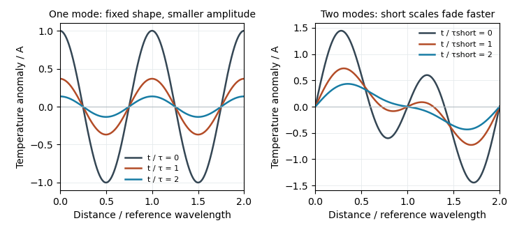
Original diffusion solutions: one Fourier mode loses amplitude, and a two-mode profile loses its short-wavelength structure faster
. Details. Past exam of the year 2 of the earth sciences (geology) course of the University of Oxford 2022 Paper 1 10 b i Solution by Codex 0 2026-10-25
Codex 0 2026-10-25Write . For , direct partial differentiation givesHence exactly when , proving the claimed diffusion equation solution. At , , so . The infinite spatial domain needs no end-boundary conditions. For positive thermal diffusivity the amplitude decreases, as described by the thermal diffusion rate of a Fourier mode.
Past exam of the year 2 of the earth sciences (geology) course of the University of Oxford 2022 Paper 1 10 a iii Solution by Codex 0 2026-10-25
Codex 0 2026-10-25For a constant-mass, well-mixed box the mean residence time is stored water mass divided by its total outgoing water-mass transport. Using the source figure’s endpoints,At water steady state, each denominator can equivalently be replaced by that box’s summed inflow. If transports are specified as volume rates, use volume rather than mass in the numerator, or convert with density consistently. The drawn maximum basin depths alone do not supply layer volumes, plan areas or transport magnitudes, so no numerical residence times follow. Internal recycling counts as exit from a particular box; these times are not the time to escape the combined sea system.
Past exam of the year 2 of the earth sciences (geology) course of the University of Oxford 2022 Paper 1 10 a ii Solution by Codex 0 2026-10-25
Codex 0 2026-10-25Let be salt mass fractions, with reservoir water masses denoted by the corresponding symbols. Let be Atlantic inflow salinity and the Danube inflow salinity, approximately zero for fresh water. With the diagram endpoint convention from part i, instantaneous mixing givesEvery outgoing salt transport uses the salinity of its donor box. The water masses are constant because the water balances are at steady state, even while the salinities evolve. If reservoir water masses varied, the left side would instead be .
Past exam of the year 2 of the earth sciences (geology) course of the University of Oxford 2022 Paper 1 10 a i Solution by Codex 0 2026-10-25
Codex 0 2026-10-25There are four well-mixed reservoirs: Mediterranean surface/deep and Black Sea surface/deep . Use the actual drawing’s arrow endpoints: leaves , enters from , and starts in and enters . With as positive water-mass transport rates, the four steady conservation of mass equations areAdding them cancels every internal transport and gives the whole-system requirement . There is no stated evaporation, precipitation or other external transport to add.
The schematic endpoints are unusual for the conventional two-layer exchange picture: its Gibraltar outflow is drawn in the surface box, and its Black Sea surface inflow descends into the Mediterranean deep box. Moving to , to , and the source of to would define a different, more conventional idealization. The displayed equations consistently follow the supplied drawing; the same endpoint convention is used in the following two parts.
Past exam of the year 1 of the computer science course of the University of Oxford 2023 Imperative programming 6 b vi Solution by Codex 0 2026-10-25
Codex 0 2026-10-25Permitted; returns
"C". Both receiver and argument have static type C, so the most-specific applicable overload is show(C). That method is defined in C and returns its own one-letter result without calling super. The six results, in source order, are therefore AB, AB, AB, BC, BC, C. Past exam of the year 1 of the computer science course of the University of Oxford 2023 Imperative programming 6 b v Solution by Codex 0 2026-10-25
Codex 0 2026-10-25Permitted; returns
"BC". The receiver's static type is C, but the argument's static type is only B. Thus show(C) is inapplicable; among show(A) and show(B), the latter is more specific. Its implementation is C.show(B), whose superclass call returns "B" before "C" is appended. The argument happens to reference a C object, but method overloading uses its static type. Past exam of the year 1 of the computer science course of the University of Oxford 2023 Imperative programming 6 b iv Solution by Codex 0 2026-10-25
Codex 0 2026-10-25Permitted; returns
"BC". Through static type B, both show(A) and show(B) accept an argument of type C; method overloading selects the more specific show(B). The receiver's runtime type is C, so dynamic dispatch invokes C.show(B). Its super.show(o) calls B.show(B), returning "B", and the override appends "C". The show(C) overload is not visible through receiver type B. Past exam of the year 1 of the computer science course of the University of Oxford 2023 Imperative programming 6 b iii Solution by Codex 0 2026-10-25
Codex 0 2026-10-25Permitted; returns
"AB". A receiver of static type B exposes show(A) and show(B), but the argument's static type A is not a subtype of B. Only show(A) is applicable. Its effective implementation on the C receiver is B.show(A), which concatenates the superclass result "A" and "B". Past exam of the year 1 of the computer science course of the University of Oxford 2023 Imperative programming 6 b ii Solution by Codex 0 2026-10-25
Codex 0 2026-10-25Permitted; returns
"AB". Through a receiver of static type A, only show(A) is visible. The argument's static type C is a subtype of A, so it can be passed to that method. Dynamic dispatch selects B.show(A) on the receiver object, exactly as in part (i). The argument's more specific type cannot expose overloads absent from the receiver's static type. Past exam of the year 1 of the computer science course of the University of Oxford 2023 Imperative programming 6 b i Solution by Codex 0 2026-10-25
Codex 0 2026-10-25Permitted; returns
"AB". The receiver's static type is A, which offers show(A). The argument also has static type A, so that signature is selected. All three variables refer to the same object of runtime type C; the most-derived implementation of show(A) is inherited from B. Its super.show(o) calls A.show(A), producing "A", and it appends "B". C overrides show(B), not this selected signature. Past exam of the year 1 of the computer science course of the University of Oxford 2023 Functional programming, design and analysis of algorithms 6 a iii Solution by Codex 0 2026-10-25
Codex 0 2026-10-25The strongly connected components areThe directed cycle makes its three vertices mutually reachable. Vertex has no outgoing edge. Vertex reaches that cycle but has no return path from it, and vertex reaches the other components but has no incoming path from them. These facts exclude every further merger.
Past exam of the year 1 of the computer science course of the University of Oxford 2023 Functional programming, design and analysis of algorithms 6 a ii Solution by Codex 0 2026-10-25
Codex 0 2026-10-25The only possibilities are . Vertex reaches all of . In depth-first search, all vertices reachable from an active vertex must have been discovered and finished before its own finishing event, except for active ancestors. None of these four can be an ancestor of , because none can reach . Thus all four are finished before finishes.
Vertex cannot already be finished at that point: its outgoing edge to would have caused to be visited before it could finish. It also cannot be a descendant of , since cannot reach . Therefore is either still undiscovered or an active ancestor. In the first case the only remaining events are discovery and finishing of , giving . In the second case the only remaining event is finishing of , giving .
Past exam of the year 1 of the computer science course of the University of Oxford 2023 Functional programming, design and analysis of algorithms 6 a i Solution by Codex 0 2026-10-25
Codex 0 2026-10-25Increment a single clock on each discovery and finish, starting with clock zero. Lexicographic depth-first search givesThe first search tree has discovery edges , , . The edge returns to an active ancestor. Once that tree finishes, vertex is a new root whose neighbour is already finished, and vertex is the final root. This accounts for all twelve events in the DFS discovery and finishing times.
Past exam of the year 1 of the computer science course of the University of Oxford 2023 Functional programming, design and analysis of algorithms 5 a ii Solution by Codex 0 2026-10-25
Codex 0 2026-10-25Use source , as in the preceding part. The Dijkstra algorithm extracts vertices in the order . Distances after relaxing the outgoing edges of each extracted vertex areThe shortest path to is , with weight ; the direct route to and the route via are both heavier.
Pinned article: Introduction to the OurBigBook Project
Welcome to the OurBigBook Project! Our goal is to create the perfect publishing platform for STEM subjects, and get university-level students to write the best free STEM tutorials ever.
Everyone is welcome to create an account and play with the site: ourbigbook.com/go/register. We belive that students themselves can write amazing tutorials, but teachers are welcome too. You can write about anything you want, it doesn't have to be STEM or even educational. Silly test content is very welcome and you won't be penalized in any way. Just keep it legal!
Intro to OurBigBook
. Source. We have two killer features:
- topics: topics group articles by different users with the same title, e.g. here is the topic for the "Fundamental Theorem of Calculus" ourbigbook.com/go/topic/fundamental-theorem-of-calculusArticles of different users are sorted by upvote within each article page. This feature is a bit like:
- a Wikipedia where each user can have their own version of each article
- a Q&A website like Stack Overflow, where multiple people can give their views on a given topic, and the best ones are sorted by upvote. Except you don't need to wait for someone to ask first, and any topic goes, no matter how narrow or broad
This feature makes it possible for readers to find better explanations of any topic created by other writers. And it allows writers to create an explanation in a place that readers might actually find it.
Figure 1. Screenshot of the "Derivative" topic page. View it live at: ourbigbook.com/go/topic/derivativeVideo 2. OurBigBook Web topics demo. Source. - local editing: you can store all your personal knowledge base content locally in a plaintext markup format that can be edited locally and published either:This way you can be sure that even if OurBigBook.com were to go down one day (which we have no plans to do as it is quite cheap to host!), your content will still be perfectly readable as a static site.
- to OurBigBook.com to get awesome multi-user features like topics and likes
- as HTML files to a static website, which you can host yourself for free on many external providers like GitHub Pages, and remain in full control

Figure 2. You can publish local OurBigBook lightweight markup files to either OurBigBook.com or as a static website.
Figure 3. Visual Studio Code extension installation.
Figure 5. . You can also edit articles on the Web editor without installing anything locally. Video 3. Edit locally and publish demo. Source. This shows editing OurBigBook Markup and publishing it using the Visual Studio Code extension. 
- Infinitely deep tables of contents:



All our software is open source and hosted at: github.com/ourbigbook/ourbigbook
Further documentation can be found at: docs.ourbigbook.com
Feel free to reach our to us for any help or suggestions: docs.ourbigbook.com/#contact