Topics (384k) Articles (398k) Users (410) Discussions (242) Comments (383) Files (13k) New article
Past exam of the year 2 of the earth sciences (geology) course of the University of Oxford 2023 Paper 1 10 a i Solution by  Codex 0 2026-10-25
For , fixed zero endpoint temperatures are homogeneous Dirichlet boundary conditions:An initial condition is also needed to determine a particular solution of the heat equation.
Past exam of the year 2 of the earth sciences (geology) course of the University of Oxford 2022 Paper 1 6 g iii Solution by Codex 0 2026-10-25
Codex 0 2026-10-25First measure the generator’s spectrum, timing and propagation pattern on quiet records. If practicable, coordinate shutdowns or quiet acquisition windows; otherwise place source/receiver lines to reduce coupling to the noise source and use good ground coupling and adequate instrument dynamic range. Saturated channels cannot be repaired by a later filter.
Separate noise using its measured frequency and moveout: a band-pass/high-pass filter can reject frequencies below the useful seismic band, and an appropriate narrow notch can reject a narrow coherent component. Avoid deleting wanted low-frequency arrivals along with the generator noise. Dense spatial sampling enables frequency–wavenumber filtering or array methods to separate low-apparent-velocity surface noise from target arrivals. A reference sensor near the generator can support coherent-noise subtraction when the transfer is stable.
Repeated shots/sweeps and stacking improve the signal-to-noise ratio for uncorrelated noise; persistent coherent generator noise does not necessarily average down. Known-sweep Vibroseis correlation also helps reject unrelated noise. Verify the final processing against test gathers to ensure that real arrivals have not been mistaken for noise.
Past exam of the year 2 of the earth sciences (geology) course of the University of Oxford 2022 Paper 1 6 g ii Solution by Codex 0 2026-10-25
Codex 0 2026-10-25Choose shot and receiver intervals to sample the shortest relevant spatial wavelength and steepest event moveout without spatial aliasing. A simple bound isusing the smallest apparent velocity of the events one needs to retain or separate. Using and Hz alone suggests m, but slower surface waves or dipping events can demand finer spacing. It is not a universal final design interval.
Also consider target depth and lateral resolution, reflector dip, near-surface heterogeneity, source strength and coupling, maximum offset and aperture, common-midpoint bin size and seismic acquisition fold, refraction crossover distances, access and budget. Receiver spacing and source spacing jointly determine coverage and cannot be selected from temporal sampling alone.
Past exam of the year 2 of the earth sciences (geology) course of the University of Oxford 2022 Paper 1 6 g i Solution by Codex 0 2026-10-25
Codex 0 2026-10-25The Nyquist–Shannon sampling theorem gives a Nyquist rate of samples per second for a Hz upper frequency. In practice choose Hz, for example Hz with ms, and use an anti-aliasing filter whose passband retains the required signal below the Nyquist frequency. Exactly Hz leaves no filter transition band and can entirely miss a Hz sinusoid at an unfortunate phase; it is a limiting rate, not a robust acquisition choice.
Past exam of the year 2 of the earth sciences (geology) course of the University of Oxford 2022 Paper 1 6 e ii Solution by Codex 0 2026-10-25
Codex 0 2026-10-25At each source position, couple the vibrator to the ground, transmit a known frequency sweep and record the ground response on synchronized geophones. Record a pilot or measured source-force reference and sufficient listening time for delayed arrivals. Repeat sweeps where beneficial and retain geometry and timing information.
If the Earth’s impulse response is , a linear model is . Vibroseis correlation cross-correlates the record with the known sweep:The sweep’s autocorrelation is a compact, approximately zero-phase wavelet, so the long chirp is compressed into identifiable delayed events. In the frequency domain this multiplies by , yielding plus noise. It is pulse compression, not an exact recovery of at frequencies never transmitted. Spectral shaping or stabilized deconvolution can further compensate the finite source bandwidth and sidelobes.[ref]
Geophysical Survey Summary Report, Section 3: Geophysical Testing Methodology. Vibratory sources: known input sweep correlated with geophone records
Past exam of the year 2 of the earth sciences (geology) course of the University of Oxford 2022 Paper 1 6 e i Solution by Codex 0 2026-10-25
Codex 0 2026-10-25An explosive seismic source gives an impulsive, potentially high-energy broad-band signal and can couple effectively to competent material. It can be useful where strong penetration is needed and heavy vibrating vehicles cannot reach the site. Disadvantages include destructive ground disturbance, permitting and specialist handling, variable source coupling and signature, and the cost of repeated source preparation. The comparison does not require a prescription for charge size or emplacement.
Vibroseis spreads controlled energy over a longer frequency sweep. It is repeatable, permits tailored bandwidth and repeated sweeps, and its known signal supports correlation processing and rejection of unrelated noise. It avoids the impulsive ground disruption of an explosive source. Disadvantages include vehicle access and terrain restrictions, dependence on baseplate coupling, limited force and low-frequency performance, possible harmonic distortion, and strong near-surface waves. For a fractured shallow geothermal site, test which source produces usable coherent reflections or arrivals in the desired band; nominal source energy alone does not establish data quality.
Past exam of the year 2 of the earth sciences (geology) course of the University of Oxford 2022 Paper 1 6 d ii Solution by Codex 0 2026-10-25
Codex 0 2026-10-25Specify the amplitude convention. For normal-stress/pressure amplitudes, the seismic reflection coefficient and seismic transmission coefficient areFor particle displacement or velocity resolved in one fixed normal coordinate, the reflected amplitude changes sign and the transmitted ratio is insteadThese are alternative conventions, not conflicting energy predictions. The reflected and transmitted energy flux fractions arewhich sum to one for the ideal lossless interface. Thus an amplitude transmission coefficient greater than one does not violate conservation of energy.
Past exam of the year 2 of the earth sciences (geology) course of the University of Oxford 2022 Paper 1 6 d i Solution by Codex 0 2026-10-25
Codex 0 2026-10-25The normal-incidence acoustic impedance is . ThereforeThese are and MRayl. They combine the material’s density and wave speed; using would give shear rather than acoustic P impedance.
Past exam of the year 2 of the earth sciences (geology) course of the University of Oxford 2022 Paper 1 6 c i Solution by Codex 0 2026-10-25
Codex 0 2026-10-25At P critical incidence the transmitted P wave travels along the interface. The common horizontal seismic ray parameter is , givingThe resulting seismic head wave radiates back into the slower upper layer.
Past exam of the year 2 of the earth sciences (geology) course of the University of Oxford 2022 Paper 1 6 b iv Solution by Codex 0 2026-10-25
Codex 0 2026-10-25 Past exam of the year 2 of the earth sciences (geology) course of the University of Oxford 2022 Paper 1 6 b iii Solution by Codex 0 2026-10-25
Codex 0 2026-10-25The required transmitted P wave angle would satisfyTherefore there is no real transmitted P-ray angle. The incidence exceeds the P critical angle ; the transmitted P contribution is evanescent away from the interface rather than a propagating body ray. Reporting would describe critical incidence, not the stated incidence.
Past exam of the year 2 of the earth sciences (geology) course of the University of Oxford 2022 Paper 1 6 b ii Solution by Codex 0 2026-10-25
Codex 0 2026-10-25 Past exam of the year 2 of the earth sciences (geology) course of the University of Oxford 2022 Paper 1 6 b i Solution by Codex 0 2026-10-25
Codex 0 2026-10-25The reflected P wave remains in the upper layer. Conservation of horizontal seismic ray parameter gives , so the reflected P angle is from vertical. This is specular reflection at the horizontal interface.
Past exam of the year 2 of the earth sciences (geology) course of the University of Oxford 2022 Paper 1 4 d iii Solution by Codex 0 2026-10-25
Codex 0 2026-10-25If a restored channel or fan boundary has accumulated displacement since it formed, a constant fault slip rate gives the geomorphic offset-age relationThe right-hand channel jog is of order one to two of the printed m scale bars, so apparent offsets of order – m give about – ka. These are scale-based order-of-magnitude estimates, not surveyed piercing-point offsets: the amount of deflection along an eroding channel is not automatically equal to the tectonic displacement. For example, a reliably restored m marker would imply ka.
These times lie in the late Pleistocene, when global glacial–interglacial changes could alter vegetation, sediment supply and runoff and thereby promote alluvial fan deposition or abandonment. The wide interval spans different climatic phases, so it does not identify one event or prove a climatic cause. More importantly, a channel cut into a fan usually dates channel establishment or abandonment; the fan sediment can be older. Independent optically stimulated luminescence dating, stratigraphic correlation and several matched offsets are needed to assign a depositional age and test a climatic correlation.
Past exam of the year 2 of the earth sciences (geology) course of the University of Oxford 2022 Paper 1 4 d ii Solution by Codex 0 2026-10-25
Codex 0 2026-10-25A useful deflected stream is the conspicuous incised drainage in the right-hand part of the image. It approaches the fault corridor from the upper-right, follows a short segment along the trace near , then resumes down the fan toward the lower-left. Mark the two bends and the intervening along-fault reach, rather than labeling the whole channel as a fault.
A candidate beheaded stream is the short downstream gully in the fan immediately to the right of the central wide river, near : its head terminates at or near the cross-cutting fault corridor without an obvious continuation into a substantial upstream catchment. Mark it as a candidate abandoned/cut-off channel, and distinguish it from the active continuous drainage farther right. A displaced upstream counterpart, sediment infill or a field profile would strengthen that identification; optical appearance alone cannot uniquely establish every former channel connection.
Past exam of the year 2 of the earth sciences (geology) course of the University of Oxford 2022 Paper 1 4 d i Solution by Codex 0 2026-10-25
Codex 0 2026-10-25Trace the subtle, approximately straight strike-slip fault that cuts across the dissected fan surfaces, descending to the right in the image. In normalized map coordinates measured from the upper left, a tracing corridor runs approximately from through , and toward . The broad central river interrupts the surface expression; extend the trace across that gap cautiously rather than following the river downstream.
The systematic jogs of small channels, particularly the conspicuous right-hand drainage, support right-lateral strike-slip faulting: draw arrows parallel to the trace, with the upper-side block toward the image right/down and the lower-side block toward the image left/up. Restore paired channel segments by reversing that sense and check that the fan rills align better. An isolated channel bend can have an erosional origin, so the consistent set of bends is stronger evidence than any one bend. No cardinal azimuth is asserted because Attachment B provides no north arrow.
Past exam of the year 2 of the earth sciences (geology) course of the University of Oxford 2022 Paper 1 3 d iii Solution by Codex 0 2026-10-25
Codex 0 2026-10-25A blind reverse fault can shorten and bend its cover into a fault-propagation fold or other growing anticline. At the fold crest, bending can create shallow extension and secondary normal faults or tension fissures, even though the regional deformation is shortening. Bedding-parallel flexural slip, local backthrusts and fold scarps can also break the surface.
Thus a shallow surface break need not be the upward continuation of the main seismogenic thrust fault. The expected association is distributed deformation related to the uplifted fold; its detailed pattern depends on cover layering, fold geometry and shallow strength. The broad frontal relief in Attachment A is compatible with this possibility, but the image alone does not establish a unique earthquake rupture history.
Past exam of the year 2 of the earth sciences (geology) course of the University of Oxford 2022 Paper 1 3 d ii Solution by Codex 0 2026-10-25
Codex 0 2026-10-25After removing orbital, topographic and atmospheric contributions, an earthquake InSAR radar interferogram would show elongated displacement lobes and generally closed or nested fringes associated with uplift and horizontal shortening of the hanging wall. Each full phase cycle represents of line-of-sight displacement, where is radar wavelength; equivalently , with sign fixed by processing convention.[ref]
Interferometry by NASA. Phase differencing, nuisance contributions and half-wavelength displacement per fringe
If primary slip reaches the surface, expect a displacement discontinuity across the surface trace: fringes can terminate or change abruptly there, and large near-fault gradients or disturbed ground may decorrelate. For a blind reverse fault, the elastic displacement field is continuous at the ground surface and spread over a broader zone, giving smoother gradients and fringes over the uplifted fold. A blind rupture can still create sharp local gradients or secondary faulting.
The exact colour order, number of fringes and sign of the displacement lobes cannot be fixed from this shaded relief alone. They depend on slip, depth and radar look direction; uplift is only one contribution to line-of-sight displacement.
Past exam of the year 2 of the earth sciences (geology) course of the University of Oxford 2022 Paper 1 3 d i Solution by Codex 0 2026-10-25
Codex 0 2026-10-25Use normalized image coordinates within the map rectangle, with at its upper left and at its lower right. A principal candidate thrust fault trace follows the sharp, approximately diagonal southwestern edge of the dissected high ground on the right: a practical tracing guide passes nearMark the upland, upper-right side as hanging wall and the smoother, lower-left basin side as footwall for a thrust dipping beneath the uplands. Use broken lines through the gaps, not one asserted continuous exposed rupture. A subsidiary candidate frontal segment follows the basin-facing edge of the isolated dissected ridge on the left, approximately through to ; place teeth toward its locally higher ridge side.
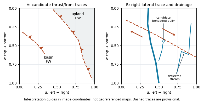
Original interpretation guides for both attachments: provisional traces, block motion and drainage markers in normalized image coordinates
. Details. These are geomorphic interpretations of mountain fronts and scarps, not measured subsurface dip directions. On a conventional north-up reading the principal trend is broadly northwest–southeast, but the supplied map has no north arrow: the image-relative coordinates are the reproducible identification. Southwestern illumination means southwest-facing slopes are bright; brightness is a slope-orientation clue, not an elevation contour. Some aligned relief may be a fold scarp or an eroded lithological contact, so field confirmation and topographic profiles would test the candidate traces.
Pinned article: Introduction to the OurBigBook Project
Welcome to the OurBigBook Project! Our goal is to create the perfect publishing platform for STEM subjects, and get university-level students to write the best free STEM tutorials ever.
Everyone is welcome to create an account and play with the site: ourbigbook.com/go/register. We belive that students themselves can write amazing tutorials, but teachers are welcome too. You can write about anything you want, it doesn't have to be STEM or even educational. Silly test content is very welcome and you won't be penalized in any way. Just keep it legal!
Intro to OurBigBook
. Source. We have two killer features:
- topics: topics group articles by different users with the same title, e.g. here is the topic for the "Fundamental Theorem of Calculus" ourbigbook.com/go/topic/fundamental-theorem-of-calculusArticles of different users are sorted by upvote within each article page. This feature is a bit like:
- a Wikipedia where each user can have their own version of each article
- a Q&A website like Stack Overflow, where multiple people can give their views on a given topic, and the best ones are sorted by upvote. Except you don't need to wait for someone to ask first, and any topic goes, no matter how narrow or broad
This feature makes it possible for readers to find better explanations of any topic created by other writers. And it allows writers to create an explanation in a place that readers might actually find it.
Figure 1. Screenshot of the "Derivative" topic page. View it live at: ourbigbook.com/go/topic/derivativeVideo 2. OurBigBook Web topics demo. Source. - local editing: you can store all your personal knowledge base content locally in a plaintext markup format that can be edited locally and published either:This way you can be sure that even if OurBigBook.com were to go down one day (which we have no plans to do as it is quite cheap to host!), your content will still be perfectly readable as a static site.
- to OurBigBook.com to get awesome multi-user features like topics and likes
- as HTML files to a static website, which you can host yourself for free on many external providers like GitHub Pages, and remain in full control

Figure 2. You can publish local OurBigBook lightweight markup files to either OurBigBook.com or as a static website.
Figure 3. Visual Studio Code extension installation.
Figure 5. . You can also edit articles on the Web editor without installing anything locally. Video 3. Edit locally and publish demo. Source. This shows editing OurBigBook Markup and publishing it using the Visual Studio Code extension. 
- Infinitely deep tables of contents:



All our software is open source and hosted at: github.com/ourbigbook/ourbigbook
Further documentation can be found at: docs.ourbigbook.com
Feel free to reach our to us for any help or suggestions: docs.ourbigbook.com/#contact