The positive and negative contributions to the integral cancel. Hence the mean is $0\mathrm{V}$.

The shorter, stronger northern pulses and broader southern pulses suggest propagation from south to north, towards the northern station. The useful evidence is the difference in pulse widths, not just the earlier northern arrivals: the latter chiefly reflect station distance.

As rupture reaches successively more northerly patches, each patch radiates a new P wave and S wave pulse. Towards the north, the later emission time is partly cancelled by a shorter propagation path; those contributions arrive closer together. Towards the south, later emission and a longer path add, stretching the signal. This is rupture directivity. It refers to the advance of the slipping region along the fault, not necessarily the direction of the local fault slip vector. A thrust can slip up-dip while its rupture front advances in a direction with a northward component.

More generally, emission from a patch at distance $s$ along the rupture arrives atThe forward direction has a smaller arrival-time spread. This is the same travel-time compression captured by isochrone-based rupture directivity calculations.^[ref] Larger northern amplitude supports the interpretation but is not decisive on its own because geometrical spreading, seismic attenuation, seismic radiation patterns and site response also affect amplitude. With only two traces, propagation, filtering and site effects remain alternatives to test; the idealized exercise is most naturally explained by northward directivity.

For a unilateral finite-source rupture advancing at approximately constant rupture velocity $V_r$, the along-fault propagation length isThere is no supplied $V_r$ or calibrated seismic source time function, so a unique spatial extent cannot be read directly from Figure 4. For illustration, $T\sim 4\mathrm{s}$ and an assumed $V_r\sim 2.5\mathrm{km}{\mathrm{s}}^{-1}$ would give $L\sim 10\mathrm{km}$. Allowing $T\sim 4$–$5\mathrm{s}$ and assumed $V_r\sim 2$–$3\mathrm{km}{\mathrm{s}}^{-1}$ gives lengths of order 8–15 km. These are explicitly conditional scale estimates, not measured fault dimensions.

If equal-and-opposite ray geometry and phase pulse durations were known, the directivity model in solution would instead constrain a projected length,where $\psi$ is the angle between the rupture direction and the northern ray. Distinct P and S wave speeds, unknown takeoff angles, smooth pulse boundaries and the clipped southern S tail prevent a reliable independent numerical inversion here. This observation is consistent with a few-kilometre projected extent while the actual along-fault length can be larger. A rupture length is not the accumulated fault slip, the width of the whole fault plane, or the approximately 50 km station distance.

Distinguish the duration of one phase pulse from the P-to-S separation. Figure 4 shows northern pulses with most visible motion over roughly 3–4 s each, compared with roughly 4–5 s or more in the south. Reading the low-amplitude tails gives approximately 11.5–15.2 s for the northern P pulse, 17.7–20.9 s for the northern S pulse, 14.2–19.0 s for the southern P pulse, and 22.3 s to beyond the right plot boundary near 27 s for the southern S pulse. Thus the latter duration is censored by the plotting window; it should not be assigned an exact ending at 27 s. The positive-to-negative extremum separations are only about 1 s in the northern pulses, 1.3 s in the southern P pulse and 1.4 s in the southern S pulse; those much shorter numbers are not full source durations. Smooth tails have no unique onset or ending at the precision of this drawing.

A finite-source rupture has an intrinsic duration $T$ that differs from the apparent pulse duration through rupture directivity. In an ideal unilateral line-source model, neglecting local slip rise time, instrument filtering and path broadening,Here $c$ is the chosen phase wave speed and $L_{\parallel }$ is the rupture's projection along equal-and-opposite takeoff directions. Averaging corresponding full pulses in that model suggests an intrinsic timescale of roughly 4–5 s. This is an order-of-magnitude graph estimate, not an exact rupture duration; the figure does not supply a seismic source time function definition, receiver responses, phase deconvolution, or geometry sufficient to determine one uniquely. A finite local slip rise time would also contribute to the observed width.

In particular, neither 13 s nor 19 s is a rupture duration: those numbers locate phase motion on the absolute clock. The northern P–S gap of 6 s is a propagation delay rather than the rupture duration.

Use the northern S–P time, approximately $\Delta t_N=6\mathrm{s}$, rather than multiplying an absolute-clock arrival by a wave speed. For common approximately straight paths,No numerical crustal velocities are specified in Q3. If the usual illustrative crustal values $V_p=6.0\mathrm{km}{\mathrm{s}}^{-1}$ and $V_s=3.5\mathrm{km}{\mathrm{s}}^{-1}$ are adopted, the distance isThese assumed crustal speeds are unrelated to Q1's offshore layer values. They are representative rather than measurements of the Swiss column; the British Geological Survey gives broad typical crustal ranges of 5–7 km/s for P waves and 3–4 km/s for S waves.^[ref]

Using the corresponding northern central pulse times gives an effective source time near $13.3-50.4/6\simeq 4.9\mathrm{s}$ after midnight, and the S estimate is the same to graph accuracy. The southern central landmarks similarly give a distance near 70 km and an effective source time near 5 s. That consistency supports the example, but pulse landmarks need not mark the rupture's true onset. $D_N$ is a source-to-station path or hypocentral distance in the uniform-speed approximation. An epicentral distance additionally needs the hypocenter depth; it cannot simply be equated to 50 km for an unknown depth.

The northern station is closer, under comparable P wave and S wave paths through the same velocity model. In the actual Figure 4 the northern P and S pulses are separated by about 6 s, whereas the southern separation is roughly 8–8.5 s. The S–P time removes the unknown earthquake origin time:Both northern pulses also occur earlier on the shared absolute clock, consistent with the smaller distance. Earlier arrival alone would not be sufficient if clocks or velocity models differed.

For reproducible graph readings, the northern positive-to-negative zero crossings are approximately $13.3\mathrm{s}$ for P and $19.3\mathrm{s}$ for S; the southern crossings are approximately $16.7\mathrm{s}$ and $25.0\mathrm{s}$. These are convenient corresponding pulse landmarks, not sharply defined first-break onsets. The first visible motion begins earlier: approximately 12 s and 18 s in the north, and 14–15 s and 22–23 s in the south, depending on the amplitude threshold. The horizontal axis is seconds since midnight on 1 January 2000, not elapsed time since rupture initiation.

For the chlorite–kaolinite reaction, take water and both solids to have unit thermodynamic activity. Its reaction quotient is $Q=a_{{\mathrm{Mg}}^{2+}}^5{a}_{{\mathrm{H}}_4\mathrm{Si}{\mathrm{O}}_4}/a_{{\mathrm{H}}^{+}}^{10}$. ThereforeThis line has a shallower negative slope than the chlorite–gibbsite line, with points $(0,12.228)$ and $(-5,13.228)$. Plot both against predominantly negative $x$, because the dissolved silica thermodynamic activity is generally below one.

Use decimal logarithms and write $x={\log }_{10}{a}_{{\mathrm{H}}_4\mathrm{Si}{\mathrm{O}}_4}$ and $y={\log }_{10}(a_{{\mathrm{Mg}}^{2+}}/a_{{\mathrm{H}}^{+}}^2)$. The question's concentration notation is interpreted as dimensionless thermodynamic activities, or concentrations divided by a fixed standard concentration with activity coefficients set to one.

For the chlorite–gibbsite reaction, unit solid activities giveHence $y=10.53-0.60x$. It is a descending straight mineral activity diagram boundary, passing through $(0,10.53)$ and $(-5,13.53)$. Its continuation alone does not establish which portions are stable against kaolinite.

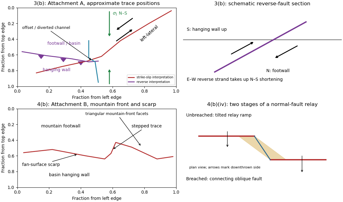
An overlapping pair of basin-dipping normal fault segments can first accommodate displacement through an unbreached relay ramp. Fault throw tapers toward each tip and transfers between the strands; the intervening block tilts and bends while retaining a continuous ramp-like surface. Draw overlapping parallel traces in plan view and a tilted connecting surface between their different fault throws.

With continued extension, the ramp can be breached by a linking fault. An oblique connector joins the segment tips and takes up a combination of dip-slip and strike-slip displacement; the system becomes a more continuous, zigzag normal fault. Draw this connector diagonally through the overlap, with downthrown arrows on the basin side. Distributed small faults and folding can accompany either arrangement. The central bend around $u\simeq 0.6$ in Attachment B is the candidate transfer zone; the image alone does not uniquely establish the three-dimensional connection at depth.

The rate of surface modification controls how quickly a fault scarp is erased. Strong rainfall, runoff, slope failure and easily eroded lithologies can round or dissect a scarp; dry conditions and resistant rock often preserve it longer. Alluvial fan deposition and aggradation can bury a scarp even if erosion is slow. A young marker surface can preserve an offset that an older, strongly modified surface no longer records.

The balance between fault slip rate, recurrence interval and marker age controls whether renewed displacement outruns this modification. Rapid or repeated normal faulting can maintain a clear front, whereas a long interval after a small displacement permits smoothing. A very young fan deposited after the event may have no offset, while an older surface may retain cumulative rather than single-event fault throw. These two controls explain why absence of an obvious scarp is not proof of an inactive fault.

Mark a fault scarp cutting an alluvial fan on the left-to-central smooth piedmont, approximately $(u,v)=(0.38,0.58)$. Its narrow, aligned height break continues across surfaces that are smoother than the mountains; repeated downthrow on the basin side produces the scarp. Sketch a once-continuous gently sloping fan surface cut by a basin-facing step.

Mark triangular facets on the mountain front in the right-central part, near $(0.78,0.48)$. These are roughly triangular planar mountain faces bounded laterally by incised valleys and below by the fault front. In a front view, draw repeated triangles separated by stream valleys. Triangular facets result from the interaction of normal faulting, uplift and erosion; neither they nor a sharp mountain front alone demonstrates a rupture in the particular historical event.

Map the continuous break near the base of the rugged mountain front, following the low scarp across the smoother fan surfaces, rather than the ridgeline. With the same normalized image coordinates, an approximate trace follows $(0.04,0.56),(0.22,0.52),(0.43,0.60),(0.55,0.64)$, steps toward $(0.62,0.43)$, and continues via $(0.72,0.49),(0.88,0.64),(0.98,0.61)$. Some parts are much clearer than others and should be drawn as inferred or dashed where obscured.

The mountainous upper side of the image is the uplifted footwall; the smoother basin/fan side below is the downthrown hanging wall. A section perpendicular to the front has a normal fault dipping toward the basin. Attachment B has no printed north arrow, so these image-relative labels avoid assigning an unsupported compass direction. The original interpretive figure marks the trace and the central fault step-over.

The network partitions deformation into oblique horizontal displacement on the strike-slip fault and more directly north–south crustal shortening on the approximately east–west reverse fault. On the oblique strand, northeastward motion of the southeastern side relative to the northwestern side has a northward component, reducing separation in the direction of ${\sigma }_1$. On the reverse fault, northward and upward motion of the southern hanging wall shortens and thickens the crust.

Sketch north–south opposing compression arrows around the plan view, left-lateral arrows along the oblique trace, and teeth on the southern side of the reverse fault trace. A section normal to the latter shows horizontal shortening converted into tectonic uplift. Where strands meet, folding, distributed strain or subsidiary faulting can maintain displacement compatibility; a strike-slip fault terminating abruptly in undeforming rock would not. This is an interpretation involving transpression, and the map does not by itself give a unique partition of slip rates between the strands.

Put the reverse fault along the mountain-front trace identified in part (ii), with the mountainous southern/southwestern block as hanging wall and the central basin to its north/northeast as footwall. Draw teeth on the southern hanging wall side of the line. In the simplest cross-section the fault dips south and the southern block moves northward and up over the basin edge. The image constrains the surface trace and relative uplift more securely than its subsurface fault dip; the precise dip cannot be measured from this map alone.

Trace the strike-slip fault along the southwest–northeast valley, approximately through $(u,v)=(0.12,0.83),(0.28,0.75),(0.44,0.68),(0.53,0.62),(0.65,0.42),(0.83,0.20),(0.97,0.04)$. The long oblique strand is interpreted as left-lateral strike-slip faulting: draw the southeastern side moving northeast and the northwestern side moving southwest, parallel to the trace.

This sense is consistent with horizontal north–south maximum compression: for an approximately northeast-striking fault, the resolved shear stress moves the southeastern side northeastward relative to the northwestern side. The deflected central drainage supports that interpretation. The regional stress direction supplies a consistency check rather than a uniquely precise trace location; follow the geomorphic break rather than drawing a single straight line through every coordinate.

A reverse fault can create a sharp mountain front by raising its hanging wall beside a lower footwall. Drainages entering the rising block may be deflected along the front or cut narrow gorges across it. In cross-section, draw a dipping fault with the hanging wall displaced up-dip and a surface-height contrast above the trace.

In Attachment A, mark the approximately east–west to west-northwest–east-southeast break between the southwestern mountain block and the central basin. Its approximate image coordinates run from $(0.03,0.56)$ through $(0.18,0.61)$ and $(0.34,0.65)$ to $(0.45,0.69)$. The abrupt topographic change and diversion of drainage along this front support the reverse faulting interpretation. It is the southern margin of the central basin, not the much straighter oblique valley farther northeast. The original interpretive figure gives a schematic section.

A displaced drainage forms when repeated horizontal fault slip offsets a channel and its upstream and downstream reaches no longer line up. In plan view, draw two initially continuous channel reaches crossing the fault, translate one side parallel to the fault strike, and connect the reaches by a short fault-parallel reach. A linear valley develops where erosion follows damaged rock along a straight fault zone.

In Attachment A, use the oblique, relatively straight valley running southwest–northeast through the lower centre towards the upper right. For an identifiable example, follow the central approximately north–south drainage to its bend near the southern edge of the central basin, about $(u,v)=(0.46,0.67)$, where $u$ is fraction from the left image edge and $v$ fraction from the top. Mark its deflected reach and the adjacent straight valley. The positional precision is at the level of the supplied image; establishing a numerical fault offset would require correlated piercing points and field checks.

For $T_n=A\cos (k_{n}x)e^{-\kappa k_n^{2}t}$, direct differentiation again gives ${\partial }_t{T}_n=-\kappa k_n^2{T}_n$ and ${\partial }_x^2{T}_n=-k_n^2{T}_n$. Thus it satisfies the heat equation. Moreover,vanishes at both endpoints for integer $n$, proving the homogeneous Neumann boundary conditions. Now $n=0$ gives the nonzero constant mode $T=A$, which does not decay. It represents conserved mean temperature in an insulated plate.

Put $k_n=n\pi /L$ and ${\lambda }_n=\kappa k_n^2$. Direct differentiation of $T_n=A\sin (k_{n}x)e^{-{\lambda }_{n}t}$ givesso ${\partial }_t{T}_n=\kappa {\partial }_x^2{T}_n$, the heat equation. At $x=0$, the sine factor vanishes; at $x=L$, it is $\sin (n\pi )=0$ for integer $n$. Thus the homogeneous Dirichlet boundary conditions hold. The nonzero, nonredundant spatial modes use $n=1,2,\dots$; $n=0$ is the zero function and negative $n$ only change the amplitude sign.

By Fourier's law, $q_x=-k{T}_x$. With nonzero thermal conductivity $k$, zero outward heat flux at both endpoints gives homogeneous Neumann boundary conditions:The outward normal has opposite signs at the two ends, but a zero-flux condition gives zero derivative at each.