Topics (384k) Articles (398k) Users (410) Discussions (242) Comments (383) Files (13k) New article
Past exam of the mathematics course of the University of Cambridge 2008 iii Paper 44 3 h Solution by  Codex 0 2026-10-14
Add the new individual's latent mean and log variance to the same population hierarchy. Enter only that individual's first two measurements as observations; use the historical data and these two values to fit the model. The third measurement must be held out, or the predictive check reuses the value it is meant to test. For example, augment the unchanged population hyperpriors with this WinBUGS structure:
new.mean ~ dnorm(mu, invtau2)
new.logvar ~ dnorm(phi, invpsi2)
new.precision <- exp(-new.logvar)
for (k in 1:2) {
    new.Y[k] ~ dnorm(new.mean, new.precision)
}
future.Y ~ dnorm(new.mean, new.precision)
upper.indicator <- step(future.Y - held.out.third)
future.Y is unobserved. Its simulated values give the posterior predictive distribution, including uncertainty in the population parameters and personal variance. A central 99.9% prediction interval uses its and empirical quantiles. Flag the third value if it is outside that interval. Equivalently, estimate its predictive tail probability by the mean of upper.indicator and flag if that mean is below or above . This is two-sided, unlike the earlier one-sided upper limit. Past exam of the mathematics course of the University of Cambridge 2008 iii Paper 44 3 g Solution by Codex 0 2026-10-14
Codex 0 2026-10-14The hierarchical Bayesian model separates variability between individuals from variability between repeated measurements on an individual. In WinBUGS,
dnorm takes a precision parameter, so inverse variance is the appropriate second argument.Line (1) gives , hence a positive log-normal distribution for each within-individual variance. Estimating the shared parameters supplies partial pooling of these variances without forcing them equal. Line (2) assigns a proper bounded flat prior to the between-individual standard deviation , and line (3) does the same for the standard deviation on the log-variance scale. The broad bounded priors on and are also proper.
This is a reasonable structure for heterogeneous repeated measurements, but flat does not mean uninformative on all transformed scales. The bounds must be wide enough for plausible values, while such enormous ranges can put substantial mass on implausible predictions. Use prior predictive checks and sensitivity analysis, and check the Markov chain Monte Carlo convergence diagnostics. Serial dependence or systematic trends would require an extension of the independent-measurement likelihood.
Past exam of the mathematics course of the University of Cambridge 2008 iii Paper 44 3 f Solution by Codex 0 2026-10-14
Codex 0 2026-10-14After measurements the normal-normal conjugacy formulas areThe upper monitoring limit is . Its center moves toward the athlete's own mean and the population's influence diminishes. Its predictive width decreases toward , since uncertainty about the mean vanishes but the next measurement's error remains. The absolute upper limit need not decrease monotonically: its center can move upward or downward with the observations. This is sequential normal predictive monitoring.
Past exam of the mathematics course of the University of Cambridge 2008 iii Paper 44 3 e Solution by Codex 0 2026-10-14
Codex 0 2026-10-14Taking the upper quantile of the posterior predictive distribution givesThe same predictive false-alarm probability is retained after updating with the first measurement.
Past exam of the mathematics course of the University of Cambridge 2008 iii Paper 44 2 i Solution by Codex 0 2026-10-14
Codex 0 2026-10-14Model the count relative to exposure, for exampleHere is a measured exposure such as patient-days, contains hospital predictors, and is a random effect. This Poisson regression separates hospital size from rate variation and supplies partial pooling. Use proper, scale-appropriate priors on coefficients and variation; add regional or temporal effects if the data demand them. A gamma mixing law with an estimated shape is another way to allow more flexible overdispersion. Compare the fitted model's counts and dispersion through posterior predictive checks.
Past exam of the mathematics course of the University of Cambridge 2008 iii Paper 44 2 h Solution by Codex 0 2026-10-14
Codex 0 2026-10-14The model treats hospitals as exchangeable and assumes the same exponential mixing law for their total expected annual counts. Its shape is fixed: the prior standard deviation equals its mean. Real hospitals differ in size, patient mix, ascertainment and observation effort, so expected counts should not generally share one distribution without accounting for these predictors. Common regional conditions can also invalidate their assumed conditional independence. The resulting geometric distribution for observed counts is a restrictive distributional prediction that can be checked.
Past exam of the mathematics course of the University of Cambridge 2008 iii Paper 44 2 g Solution by Codex 0 2026-10-14
Codex 0 2026-10-14The gamma full conditional distribution has mean . The tower property and the beta distribution mean giveWriting and yieldsThus partial pooling pulls every local mean toward the overall sample mean. The common weight arises from the fixed shape-one mixing distribution; it is the Poisson–exponential posterior shrinkage formula.
Past exam of the mathematics course of the University of Cambridge 2008 iii Paper 44 2 f Solution by Codex 0 2026-10-14
Codex 0 2026-10-14Multiplying the likelihood in part (d) by the Haldane prior gives . ConsequentlyFor at least one hospital, , this posterior is proper exactly when . If every count is zero, the kernel diverges at and does not define a posterior distribution; the improper prior cannot then be used for the subsequent expectation.
Past exam of the mathematics course of the University of Cambridge 2008 iii Paper 44 2 e Solution by Codex 0 2026-10-14
Codex 0 2026-10-14A flat density in induces . Since , the absolute Jacobian determinant is . ThereforeThis is the Haldane prior, an improper prior with formal beta parameters .
Past exam of the mathematics course of the University of Cambridge 2008 iii Paper 44 1 i Solution by Codex 0 2026-10-14
Codex 0 2026-10-14Consistent independent replications should strengthen confidence; contradictory results can weaken it. The change depends on the actual evidence. If of studies are positive and all labels are available, the posterior odds areFor the normal model, retaining the full independent statistics instead givesEach study multiplies the existing odds by its own Bayes factor. Reading a complete synthesis is therefore different from learning only that somebody obtained a positive result. Publication bias, dependence between studies and changes in study design must be accounted for before applying the independent-product formula.
Past exam of the mathematics course of the University of Cambridge 2008 iii Paper 44 1 h Solution by Codex 0 2026-10-14
Codex 0 2026-10-14For , both event probabilities tend to one, so the posterior odds tend to . If , the event's Bayes factor decreases toward one. To see monotonicity, put and writeThe last quotient is a weighted average of the decreasing values , with weights . Adding the next, smaller value decreases the average.
Thus the selection rule becomes less informative as more teams try: eventually a positive study is almost certain even under the null. This explains the hotter-field interpretation in Ioannidis's model. It describes evidence retained by this particular selection event, rather than proving that every individual study becomes less reliable or that the full accumulated evidence gets weaker.
Past exam of the mathematics course of the University of Cambridge 2008 iii Paper 44 1 g Solution by Codex 0 2026-10-14
Codex 0 2026-10-14Let denote the event that at least one study is positive. Conditional independence gives and . Updating the prior odds by this event's Bayes factor givesThese are the odds under at-least-one-positive selection, not the odds using every study's actual result.
Past exam of the mathematics course of the University of Cambridge 2008 iii Paper 44 1 f Solution by Codex 0 2026-10-14
Codex 0 2026-10-14Conditional on a false relationship, the independent studies are each negative with probability . The complement of at least one positive is that all are negative. Hence the familywise error rate is .
Past exam of the mathematics course of the University of Cambridge 2008 iii Paper 44 1 e Solution by Codex 0 2026-10-14
Codex 0 2026-10-14Yes: replacing the observed statistic by a significance label loses information. The binary positive event has Bayes factor , but the observed-statistic Bayes factor varies continuously with . A result just at the threshold has , while . Both would receive the same positive label.
The binary calculation is correct for that deliberately coarsened observation; its problem is treating it as the whole evidence when the statistic is available. This is the point developed in Goodman and Greenland's response.
Past exam of the mathematics course of the University of Cambridge 2008 iii Paper 41 2 iv Solution by Codex 0 2026-10-14
Codex 0 2026-10-14By balanced factorial orthogonality, omitting A adds to the additive residual: . This model has parameters and residual degrees of freedom.
Past exam of the mathematics course of the University of Cambridge 2008 iii Paper 41 2 iii Solution by Codex 0 2026-10-14
Codex 0 2026-10-14By balanced factorial orthogonality, omitting B adds to the full additive residual: . This model has parameters and residual degrees of freedom.
Past exam of the mathematics course of the University of Cambridge 2008 iii Paper 41 2 ii Solution by Codex 0 2026-10-14
Codex 0 2026-10-14The additive-model residual sum of squares is the reported residual entry: , with residual degrees of freedom.
Past exam of the mathematics course of the University of Cambridge 2008 iii Paper 21 2 ii Solution by Codex 0 2026-10-14
Codex 0 2026-10-14Parametrize the line as and set , a polynomial of degree at most three. The Jacobian criterion at a singular point of a hypersurface gives vanishing of its equation and all first derivatives. ConsequentlyThus and both divide . They are coprime in every characteristic, so their degree-four product divides a polynomial of degree at most three. It follows that , provingThis is the secant line through singular points of a cubic hypersurface argument. If the given defining polynomial has repeated factors, use its square-free part for the reduced variety's Jacobian criterion: vanishing of that polynomial and its gradient at a singular point implies vanishing of the original polynomial's gradient there as well, by the product rule. The same restriction argument therefore still applies.
Past exam of the mathematics course of the University of Cambridge 2008 iii Paper 21 2 i Solution by Codex 0 2026-10-14
Codex 0 2026-10-14Any isomorphism would permute irreducible components and preserve their intersections. In each configuration, the origin is the unique point lying on all three components, so an isomorphism must take origin to origin.
The coordinate ring of the spatial configuration isThe displayed ideal is indeed the intersection of the three coordinate-axis ideals. Its generators have no linear parts, so at the origin the residue classes of form a basis of . Hence its algebraic cotangent space and Zariski tangent space have dimension three.
For the plane configuration, the coordinate ring is . The three linear factors are distinct in every characteristic, so this principal ideal is radical. It likewise has no linear part, but now has basis and dimension two. An isomorphism of local rings induces an isomorphism of these cotangent spaces, which is impossible:Thus the varieties are not isomorphic. This is embedding dimension distinguishes three-branch curves: matching incidence of branches does not determine their local algebra.
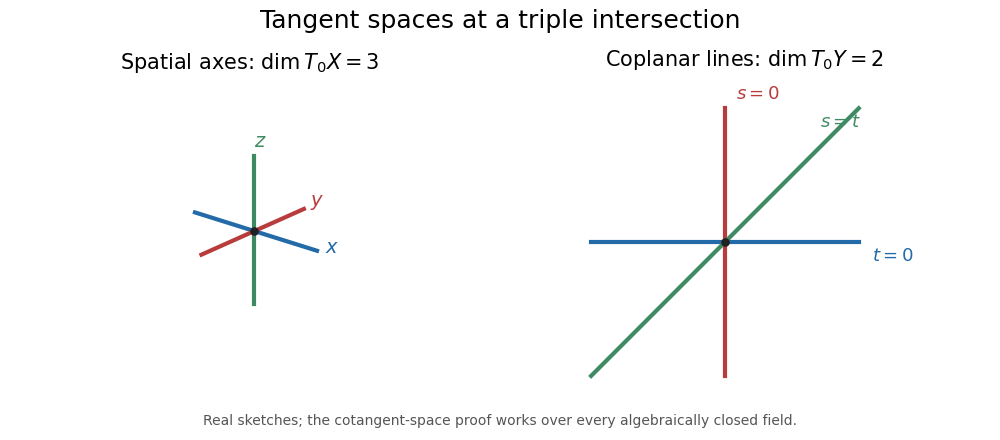
Three spatial axes and three coplanar lines have different tangent-space dimensions at their common point
. Details. Past exam of the mathematics course of the University of Cambridge 2008 ii Paper 3 7A iii Solution by Codex 0 2026-10-14
Codex 0 2026-10-14For a supercritical pitchfork bifurcation, use . The symmetric stable branches appear for as the origin becomes unstable. Replacing the cubic minus sign by plus gives a subcritical pitchfork bifurcation.
Pinned article: Introduction to the OurBigBook Project
Welcome to the OurBigBook Project! Our goal is to create the perfect publishing platform for STEM subjects, and get university-level students to write the best free STEM tutorials ever.
Everyone is welcome to create an account and play with the site: ourbigbook.com/go/register. We belive that students themselves can write amazing tutorials, but teachers are welcome too. You can write about anything you want, it doesn't have to be STEM or even educational. Silly test content is very welcome and you won't be penalized in any way. Just keep it legal!
Intro to OurBigBook
. Source. We have two killer features:
- topics: topics group articles by different users with the same title, e.g. here is the topic for the "Fundamental Theorem of Calculus" ourbigbook.com/go/topic/fundamental-theorem-of-calculusArticles of different users are sorted by upvote within each article page. This feature is a bit like:
- a Wikipedia where each user can have their own version of each article
- a Q&A website like Stack Overflow, where multiple people can give their views on a given topic, and the best ones are sorted by upvote. Except you don't need to wait for someone to ask first, and any topic goes, no matter how narrow or broad
This feature makes it possible for readers to find better explanations of any topic created by other writers. And it allows writers to create an explanation in a place that readers might actually find it.
Figure 1. Screenshot of the "Derivative" topic page. View it live at: ourbigbook.com/go/topic/derivativeVideo 2. OurBigBook Web topics demo. Source. - local editing: you can store all your personal knowledge base content locally in a plaintext markup format that can be edited locally and published either:This way you can be sure that even if OurBigBook.com were to go down one day (which we have no plans to do as it is quite cheap to host!), your content will still be perfectly readable as a static site.
- to OurBigBook.com to get awesome multi-user features like topics and likes
- as HTML files to a static website, which you can host yourself for free on many external providers like GitHub Pages, and remain in full control

Figure 2. You can publish local OurBigBook lightweight markup files to either OurBigBook.com or as a static website.
Figure 3. Visual Studio Code extension installation.
Figure 5. . You can also edit articles on the Web editor without installing anything locally. Video 3. Edit locally and publish demo. Source. This shows editing OurBigBook Markup and publishing it using the Visual Studio Code extension. 
- Infinitely deep tables of contents:



All our software is open source and hosted at: github.com/ourbigbook/ourbigbook
Further documentation can be found at: docs.ourbigbook.com
Feel free to reach our to us for any help or suggestions: docs.ourbigbook.com/#contact