Beta distribution ($\mathrm{Beta}(\alpha ,\beta )$)

The beta distribution is an absolutely continuous probability distribution for a random variable $X$ between zero and one. It can describe uncertainty about a probability, such as an unknown coin's chance of heads. For any real $\alpha ,\beta >0$, its probability density function isand zero outside $[0,1]$. The normalizer is the Euler beta function, related to the gamma function by the beta-gamma identity:Thus the probability density function integrates to one. ^[ref].

The endpoint behavior explains why the restrictions are exactly $\alpha ,\beta >0$: near zero the probability density function behaves like a constant times $x^{\alpha -1}$, and near one like a constant times $(1-x{)}^{\beta -1}$. These improper integrals converge for positive parameters, even when the probability density function diverges at zero for $\alpha <1$ or at one for $\beta <1$. There is no probability mass at either endpoint: $\mathbb{P}(X=0)=\mathbb{P}(X=1)=0$. A probability density function's height is not a probability; an interval's probability is the area under it.

Some useful examples of the beta distribution are:

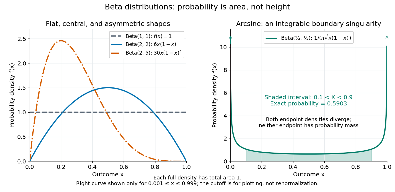
The arcsine distribution curve is plotted only for $0.001\le x\le 0.999$; its finite plotted ends do not represent finite endpoint values of the probability density function. Using the inverse sine, the shaded central interval has exact probability $\mathbb{P}(0.1<X<0.9)=1-4\arcsin (\sqrt{0.1})/\pi \approx 0.5903$, calculated analytically rather than by treating the cropped curve as normalized.

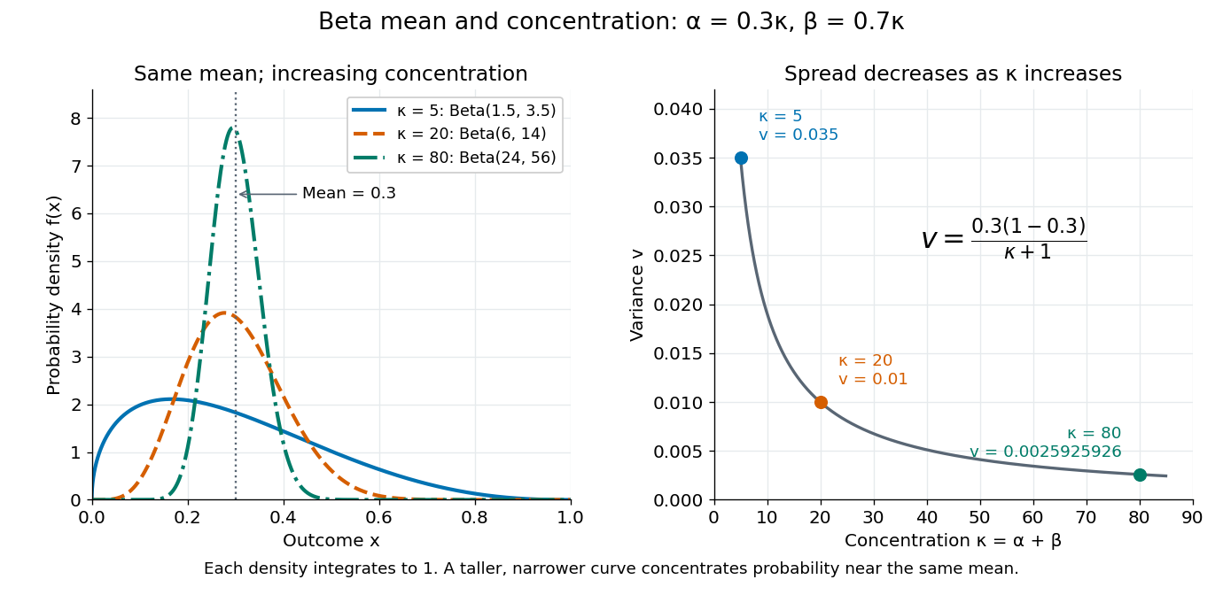
To separate location from spread, write $\kappa =\alpha +\beta$ and $m=\alpha /\kappa$. The mean and variance of the beta distribution areThe mean specifies the balance between the parameters; their sum $\kappa$ controls concentration about that mean. Multiplying both parameters by the same positive number preserves the mean and changes the variance. Larger $\kappa$ puts more area near $m$ and makes the probability density function taller there; the total area stays one. Small $\kappa$ allows much greater spread, sometimes favoring the endpoints rather than the mean itself.

For example, keeping mean $m=0.3$ and taking $\kappa =5,20,80$ gives the beta distributions $\mathrm{Beta}(1.5,3.5)$, $\mathrm{Beta}(6,14)$, and $\mathrm{Beta}(24,56)$. Their variances are $0.035$, $0.01$, and $0.21/81\approx 0.00259259$, respectively. Parameters need not be integers.

The formulas follow from two short moment calculations. Multiplying the probability density function by $x$ or $x^2$ increases the first parameter of the Euler beta function:Apply the Gamma function recurrence to the beta-gamma identity, then subtract $(\mathbb{E}[X]{)}^2$ from $\mathbb{E}[X^2]$ to obtain the variance.

The beta distribution is especially convenient as a prior distribution for the unknown success probability $P$ of Bernoulli trials. The Beta-binomial conjugacy says that $h$ successes and $t$ failures update a prior distribution $\mathrm{Beta}(\alpha ,\beta )$ to a posterior distribution $\mathrm{Beta}(\alpha +h,\beta +t)$. For example, suppose a coin has prior distribution $\mathrm{Beta}(2,2)$ and we observe eight heads and two tails. Its posterior distribution is then $\mathrm{Beta}(10,4)$, with posterior mean $5/7$. ^[ref].

For $X\sim \mathrm{Beta}(\alpha ,\beta )$ with positive parameters, and real $s>-\alpha$, $t>-\beta$, multiply its density by $x^s(1-x{)}^t$. The resulting integral is a beta function with shifted parameters, henceThe restrictions on the powers are exactly the endpoint-integrability conditions. This includes ordinary moments, reciprocal moments when they exist, and quantities involving both the occupied fraction $X$ and remaining fraction $1-X$. In particular, $s=1,t=0$ gives $\mathbb{E}[X]=\alpha /(\alpha +\beta )$.^[ref]

For $\Theta \sim \mathrm{Beta}(1,\beta )$, direct integration of its probability density function gives the displayed tail for $0<t<1$. Increasing $\beta$ strictly decreases every such tail probability, and $\Theta$ converges in probability to zero as $\beta \to \infty$. Its mean is $1/(\beta +1)$ and its variance is $\beta /[(\beta +1{)}^2(\beta +2)]$; both decrease for $\beta >1$. For the variance, logarithmic differentiation gives $1/\beta -2/(\beta +1)-1/(\beta +2)<0$ in that range.

After $S$ successes in $N$ conditionally independent Bernoulli trials, Beta-binomial conjugacy gives posterior mean $(S+1)/(N+\beta +1)$. Its derivative with respect to $\beta$ is negative, while the weight $(\beta +1)/(N+\beta +1)$ assigned to the prior mean is increasing for $N>0$.

For an independent statistical sample from the beta distribution with parameters $(\theta ,1)$, $\theta >0$, the probability density function is $\theta x^{\theta -1}$ on $(0,1)$. Its raw moments are $\mathbb{E}{X}^r=\theta /(\theta +r)$ for $r>-\theta$, by direct integration. Consequently the method of moments gives $T_1=\bar{X}/(1-\bar{X})$, whereas the maximum-likelihood estimator is $T_2=-n/{\sum }_i\log X_i$.

The second formula follows by setting the score function $n/\theta +{\sum }_i\log X_i$ to zero; its derivative is negative. Also $-\log X_i$ has an exponential distribution of rate $\theta$, since $\mathbb{P}(-\log X_i>u)=e^{-\theta u}$. The central limit theorem and delta method giveThus the asymptotic relative efficiency of $T_1$ relative to $T_2$ is $1-(\theta +1{)}^{-2}$. The transformed sum has a gamma distribution of shape $n$ and rate $\theta$, which also gives $\mathbb{E}{T}_2=n\theta /(n-1)$ for $n>1$ and $\mathrm{Var}(T_2)=n^2{\theta }^2/[(n-1{)}^2(n-2)]$ for $n>2$.

Moment matching for a beta prior turns a desired mean and variance for an unknown probability into the parameters of a beta distribution prior. Choose $0<m<1$ andSolving the beta distribution mean and variance identities givesThe strict upper bound on the variance makes $\kappa >0$, so both parameters are positive. Substitution gives mean $\mathbb{E}[P]=m$ and variance $\mathrm{Var}(P)=v$ exactly. A smaller specified variance at fixed mean produces a more concentrated prior distribution.

For example, a desired prior mean $m=0.3$ and variance $v=0.01$ give $\kappa =0.21/0.01-1=20$, hence the beta distribution prior $\mathrm{Beta}(6,14)$. With the same mean and variance $v=0.035$, the calculation instead gives $\kappa =5$ and the broader beta distribution prior $\mathrm{Beta}(1.5,3.5)$. Both appear in the concentration diagram above.

The excluded boundary cases have clear meanings. Zero variance would require $P=m$ with certainty, not a beta distribution with finite positive parameters. At the other boundary, any random variable $P\in [0,1]$ satisfies $P^2\le P$, hence variance at most $m(1-m)$; equality requires $P$ to take only the endpoint values zero and one. This is a Bernoulli distribution, not a beta distribution. Thus $v\ge m(1-m)$ cannot be matched by positive finite parameters, and $m=0$ or $m=1$ is also excluded.

After observing $n=h+t>0$ Bernoulli trials, the Beta-binomial conjugacy makes the posterior mean a weighted average of the prior mean $m$ and observed binomial proportion $h/n$:This formula gives $\kappa$ a precise interpretation as the prior's weight relative to the sample size in this posterior mean. It does not require fictitious observed counts: the beta distribution parameters can be any positive real numbers. For the eight-head, two-tail example above, $\kappa =4$ and $m=1/2$, so the posterior mean is $(4\cdot 1/2+10\cdot 0.8)/14=5/7$.

// Target: statistical-inference.bigb

For positive integers $\alpha ,\beta$, the $\alpha$th order statistic from $\alpha +\beta -1$ independent uniform distributions on $(0,1)$ has Beta distribution $\mathrm{Beta}(\alpha ,\beta )$. Selecting the observations below and above a value $u$ gives its probability density function proportional to $u^{\alpha -1}(1-u{)}^{\beta -1}$, with normalizing factor $(\alpha +\beta -1)!/((\alpha -1)!(\beta -1)!)$.

Independent gamma distributions $S\sim \Gamma (\alpha ,r)$ and $T\sim \Gamma (\beta ,r)$ with a common rate yield a Beta distribution $S/(S+T)\sim \mathrm{Beta}(\alpha ,\beta )$. The change of variables $S=wu$, $T=w(1-u)$ has Jacobian determinant $w$, and factors the joint probability density function into a Beta distribution density in $u$ and a gamma distribution density in $w$. In particular, independent chi-squared distributions with $2\alpha$ and $2\beta$ degrees of freedom give the required ratio.