Random variables and are conditionally independent given when, for every pair of Borel sets , the following identity holds almost surely:Here conditional probabilities are conditional expectations of the corresponding indicator random variables given the sigma-algebra generated by . This defines the condition even when . In terms of regular conditional distributions, the conditional joint law is the product of the conditional marginal distributions for almost every conditioning value.
For discrete random variables, at every with , the condition becomesWhere , this is equivalent to . Once is known, observing provides no further information about .[ref]
Information Theory I — Scene Setting and Statistical Applications (Lecture 9). Information Theory I — Scene Setting and Statistical Applications, Lecture 9, section Conditional independence and conditional mutual information: conditional factorization and predictive irrelevance
For a worked example, suppose a latent variable chooses between two environments with . Given , take to be independent and identically distributed with a Bernoulli distribution of parameter , where and . Think of two separate trials run under the same quiet or active environment. Their conditional joint probability mass functions, with rows and columns , areEach is exactly the product of its own conditional marginal distributions: for , and for . Thus are conditionally independent given .
If the environment is unobserved, the law of total probability averages the two tables:Both unconditional marginal distributions are fair, but . The law of total expectation gives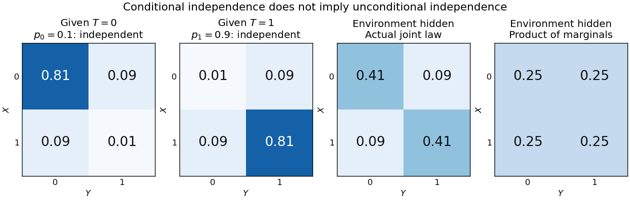
Figure 1.
An unobserved shared environment creates statistical dependence between conditionally independent trials
. The first two tables show independent Bernoulli trials at conditional success probabilities and . Averaging them with equal weights gives the third table. The fourth table is the product of the resulting unconditional marginal distributions, which differs from the actual joint table. These are stipulated model probabilities, not observed frequencies. Details.
Observing makes the active environment more plausible, so it raises to . Knowing the actual environment removes this source of statistical dependence. The covariance induced by a shared latent variable lemma explains the calculation without listing all the outcomes.
This is why conditional independence is useful in statistical modelling: a model can multiply simple conditional laws and then average over a shared latent variable. The resulting observations can remain statistically dependent. Conditional independence graphs organize such information relations; their interpretation as causes requires additional assumptions from causal inference. Conditioning describes the information available to an observer. It does not, by itself, describe what would happen if an experimenter changed a variable.
Return to pairwise independence does not imply joint independence, where are independent fair bits and is their exclusive or. Given , only and remain, each with conditional probability . Given , only and remain, again each with conditional probability . Consequently,The conditional marginal distributions are still fair, so their product has four entries in either case. The actual tables differ: given , and given . Thus unconditional independence need not survive conditioning. Observing whether two bits agree restricts their possible combinations; no physical interaction between the original trials is required to produce that information constraint.
Let be independent random variables, each with a Bernoulli distribution of parameter , and put . Unconditionally, the four ordered pairs each have probability . On the event , only and remain, each with conditional probability . ThusKnowing that exactly one trial succeeded makes observing one outcome informative about the other. This violates conditional independence given , even though the original random variables are independent. Given or , both variables are constant random variables and are conditionally independent there; that does not repair the failure at , an event of positive probability.
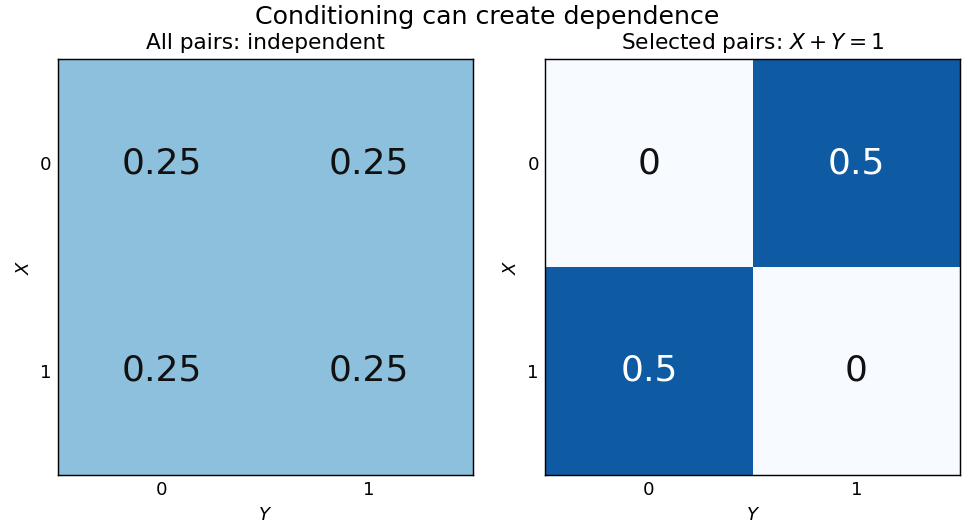
Selecting pairs with exactly one success makes independent trials dependent
. Left: four equally probable outcomes of independent fair Bernoulli trials. The selection retains exactly two pairs. Right: their conditional joint table has zero mass on the diagonal and off it. Within this selected model the conditional covariance is ; the two conditional marginal distributions remain fair. Details.
The conditional covariance here is . Both conditional variances are , so the conditional correlation coefficient is : within the selected group, . These conclusions follow from restricting a finite sample space, without positing any physical interaction between the trials.
This example and the shared-environment example establish both logical directions: independent random variables need not be conditionally independent, and conditionally independent variables need not be independent. When is represented as the joint result of two inputs in a causal directed acyclic graph, conditioning on it has the collider structure associated with collider bias. A probability calculation by itself establishes a dependence relation, not a physical causal mechanism or an intervention.
For a random vector indexed by vertices , its conditional independence graph is the undirected graph with absent exactly when . In a nonsingular multivariate normal distribution, its edges are the nonzero off-diagonal entries of the precision matrix.
Fit the conditional law of each variable given all others and use its predictor support to estimate its neighbours. In a Gaussian graphical model, this is linear regression with coefficients given by conditional regression coefficients from a Gaussian precision matrix. The Nodewise Lasso supplies sparse fits; the OR rule for nodewise graph selection and AND rule for nodewise graph selection combine possibly disagreeing directional supports into an undirected graph.
Minimizing the squared error over each free regression intercept gives the displayed formula. Substitution replaces all data columns by centred columns. The regression intercept is generally not the marginal mean of the response when predictor means are nonzero; the distinction matters in conditional regression coefficients from a Gaussian precision matrix.
The intersection rule retains an edge only when both directions of nodewise regression select it. It is more conservative than the OR rule for nodewise graph selection; the distinction matters because separate finite-sample fits can disagree.
The union rule retains an edge whenever either of the two nodewise regression fits selects the other variable. It is more inclusive than the AND rule for nodewise graph selection and makes an undirected edge decision from potentially asymmetric estimated neighbourhoods.
For a nondegenerate multivariate normal distribution, the conditional independence graph is read from zeros in its precision matrix. Conditional independence of two components given all others is equivalent to a zero cross term in their conditional Gaussian quadratic density, hence to . It does not generally correspond to a zero in the covariance matrix.
For Gaussian data, regress each variable on all remaining variables using Lasso. Nonzero coefficients estimate its neighbours in the conditional independence graph. Symmetrize the separate regressions using either the union or the intersection of their selected directed neighbourhoods.
If D-separation and conditional independence are equivalent for a Directed acyclic graph, its moral graph is its conditional independence graph. After conditioning on all other vertices, an active path can only be a direct edge or a two-edge collider through a common child: two adjacent interior vertices cannot both be colliders. These are exactly the moral edges.
The contraction axiom says thatIt follows directly by multiplying the corresponding conditional-density factorizations.
The decomposition axiom says that implies both and . It follows by marginalizing the joint conditional distribution over the discarded variable.
To test , regress and on and average the products of their residuals. Dividing the scaled average by its empirical second moment produces the generalized covariance measure statistic. Small mean-square nuisance-regression errors and a product-rate condition make it asymptotically pivotal.
If the numerator of the generalized covariance measure statistic obeys a central limit theorem with variance and its empirical residual-product second moment converges in probability to the same positive quantity, the Slutsky theorem makes the studentized statistic converge in distribution to .
Articles by others on the same topic
There are currently no matching articles.