Topics (384k) Articles (398k) Users (410) Discussions (242) Comments (383) Files (13k) New article
Past exam of the mathematics course of the University of Cambridge 2007 iii Paper 85 1 a Solution by  Codex 0 2026-10-14
Put and extend the system by . At the zero equilibrium with zero parameters, the block is the nilpotent matrix , while the eigenvalues are . Since , these are stable. The extended centre manifold is a graph , tangent to the four-dimensional centre space containing the two parameter directions. Its invariance equations areFor the quadratic jets in the ordinary total degree, the coefficient multiplying has no linear part. Hence and . With , comparison gives , , . The second graph is obtained in the same way. Terms involving parameters at quadratic order have zero forcing and vanish. Thus the quadratic centre manifold for a pair of linear filters isSubstitution into the centre equations gives the cubic termsThe last displayed cubic term is absent from the proposed second-order approximation, so its omission needs the weighted scaling rather than an ordinary-degree truncation.
Under the hinted scaling , , , , one has and . The invariance equations at weighted orders two and three give and . In particular no additional parameter-dependent weighted-order-three graph terms appear. Therefore the term and the omitted manifold corrections affect the reduced acceleration only at order , whereas has order and order . After division by , the slow equation isThis proves why the stated approximation retains the leading nonlinear restoring force and its first nonlinear damping correction. The centre manifold theorem removes the exponentially decaying transverse directions, while the retained generic coefficients determine the nearby reduced bifurcations. It is a local asymptotic description, not an exact global reduction. If either relevant coefficient vanishes, higher-order terms may be needed to resolve that degeneracy; the two extreme cases in part (b), with , avoid it.
Past exam of the mathematics course of the University of Cambridge 2007 iii Paper 77 1 ii Solution by Codex 0 2026-10-14
Codex 0 2026-10-14For , the dispersion relation gives . Put . Boundedness as selects , rather than the exponentially growing root. The internal-wave polarization relations now yieldAgain take real parts and set . This is an evanescent wave, decaying over distance ; there is no propagating far-field internal gravity wave at this frequency. The pressure amplitude is in quadrature with the horizontal velocity, so the time-averaged horizontal pressure-work flux vanishes. The equality is a singular limiting case and is outside the two frequency ranges considered here.
Past exam of the mathematics course of the University of Cambridge 2007 iii Paper 50 3 d Solution by Codex 0 2026-10-14
Codex 0 2026-10-14At order , scalar particle–antiparticle scattering has a -channel photon exchange and an -channel annihilation and recreation diagram. They are shown below, with incoming momenta and outgoing momenta . The seagull vertex has only two scalar legs and does not yield a four-scalar tree diagram at this order.
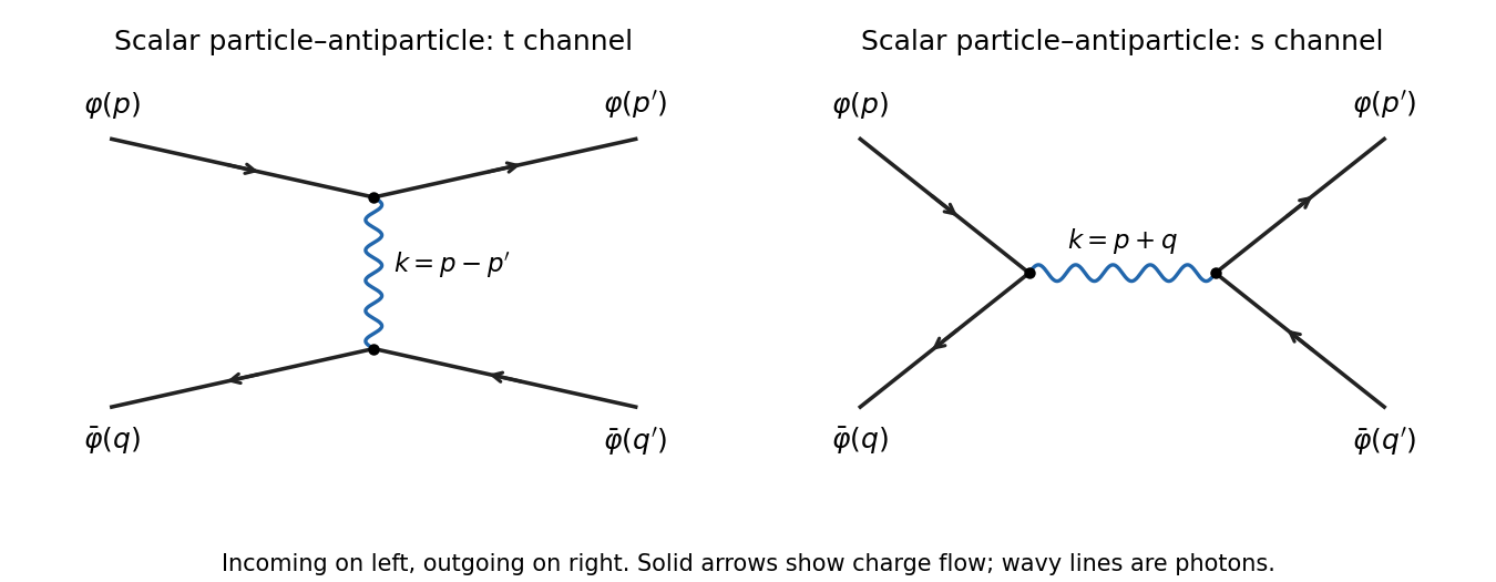
Leading scalar particle–antiparticle scattering diagrams with exchanged and annihilation-channel photons
. Details. For the exchange graph, let . Apart from overall charge signs, the two scalar currents are and . The external mass shell conditions giveFor the annihilation graph, , with currents and , again up to vertex signs. Their contractions are and . Thus each graph couples the photon to conserved currents, the relevant scalar quantum electrodynamics Ward identity.
Write and . conserved current means and . For , contraction with the Coulomb-gauge photon propagator gives, displaying the rational identity before the pole boundary limit,We used . Restoring the common Feynman i-epsilon prescription yields the Coulomb-gauge propagator between conserved currents resultHence each on-shell tree amplitude can use the Lorentz-invariant propagator. This is equality after contraction, not equality of the gauge-dependent tensors. At , the separate Coulomb-gauge terms are ill-defined; combine them first and take the conserved-current limit. The combined expression has only the physical photon pole.
Past exam of the mathematics course of the University of Cambridge 2007 iii Paper 50 3 c Solution by Codex 0 2026-10-14
Codex 0 2026-10-14Expand the gauge covariant derivative in the scalar kinetic term:The cubic interaction is thereforeFor an incoming scalar momentum and outgoing momentum , derivatives give on the incoming field and on its outgoing conjugate. Multiplication by the factor from the interaction action gives the scalar electrodynamics three-point vertex .
The other vertex comes fromDifferentiating twice with respect to the identical photon fields gives a factor of two, so the seagull vertex is . There is no additional factor of two from the scalar fields, since the complex scalar field and its conjugate are distinct legs.
Past exam of the mathematics course of the University of Cambridge 2007 iii Paper 50 3 b Solution by Codex 0 2026-10-14
Codex 0 2026-10-14A gauge redundancy relates different field representatives of the same physical configuration. For example, the transformation just exhibited changes and the scalar phase but leaves , and all other gauge-invariant operators unchanged. Fixing a gauge removes this freedom; it does not remove a physical symmetry-related state. In canonical quantization, local transformations trivial at the boundary are generated by the Gauss law constraint in gauge theory, and physical states satisfy that constraint.
A global symmetry in field theory instead has a spacetime-independent parameter and can act nontrivially on physical states. For a continuous global symmetry in field theory, Noether theorem gives a conserved charge that generates the transformation and labels the states; discrete global symmetries do not acquire a Noether current from the same infinitesimal theorem. These are statements about physical transformations, rather than merely whether a parameter is written as a constant or a function.
Boundary conditions matter in gauge theory. gauge transformations that vanish at spatial infinity are redundancies, while transformations nontrivial at infinity may act through a physical electric charge. In particular a constant phase transformation can survive as a global charge symmetry rather than being quotiented out with the local gauge redundancy. Thus local gauge redundancy is a redundancy of description; genuine global symmetry in field theory can distinguish physical states and charges, with the boundary qualification made explicit.
Past exam of the mathematics course of the University of Cambridge 2007 iii Paper 50 3 a Solution by Codex 0 2026-10-14
Codex 0 2026-10-14For any real smooth function , make the local transformationThe electromagnetic field tensor is unchanged because the mixed derivatives of commute. Directly,Its conjugate transforms with the inverse phase, so is invariant. The mass term depends only on and is invariant as well. All terms of the action are therefore unchanged. This proves the local U(1) gauge symmetry of scalar electrodynamics.
Past exam of the mathematics course of the University of Cambridge 2007 iii Paper 5 3 iii Solution by Codex 0 2026-10-14
Codex 0 2026-10-14Suppose first that is uniform and is a powerful open subgroup. The torsion criterion stated above makes a torsion-free group; so is a torsion-free group too. It is finitely generated, for example by the Schreier lemma, and hence is uniform by the same criterion. Put and , and choose with . For every ,Uniformity of the two groups givesTaking logarithms and dividing by , then letting , proves . This proves (i)(iii) without assuming that is a power subgroup. Conversely every is powerful and open, so (iii) applied to these subgroups gives (ii). Therefore all three conditions are equivalent.
The remaining nested parts establish the stated properties of the transported operations defined in the root solution.
Past exam of the mathematics course of the University of Cambridge 2007 iii Paper 47 4 b Solution by Codex 0 2026-10-14
Codex 0 2026-10-14A metric dissimilarity must satisfy, for all , the four propertiesThey are nonnegativity, identity of indiscernibles, symmetry and the triangle inequality. The following two transformations of the simple matching coefficient behave differently at the identity.
Past exam of the mathematics course of the University of Cambridge 2007 iii Paper 32 1 iii Solution by Codex 0 2026-10-14
Codex 0 2026-10-14Euclidean Lipschitz continuity does not imply Carnot-Carathéodory Lipschitz continuity. In the exponential coordinates above take the vertical path . It is Euclidean Lipschitz continuous, butIndeed left invariance reduces to the central increment, graded dilation gives the square-root factor, and reversal changes the sign without changing the distance.
One can also see the scale directly. A horizontal curve starting at the identity satisfies . If it ends on the vertical axis, its planar projection is a closed loop andFor a projection of length starting at zero, , so . Thus reaching a central displacement requires length at least , while a square loop with the appropriate signed area gives length at most . In particular is unbounded as . Vertical displacement records area, which scales quadratically with horizontal length.
Past exam of the mathematics course of the University of Cambridge 2007 iii Paper 32 1 ii Solution by Codex 0 2026-10-14
Codex 0 2026-10-14For with basis , the step-two Lie algebra has basis and its last element is central. WriteIts first level is and its second level isThe step-two multiplication givesConsequently the mapis an isomorphism onto the real Heisenberg group. The shift by converts exponential coordinates into the matrix coordinates used for that group. In exponential coordinates the left-invariant horizontal vector fields areTaking orthonormal gives exactly the Carnot-Carathéodory distance inherited from .
Past exam of the mathematics course of the University of Cambridge 2007 iii Paper 32 1 i Solution by Codex 0 2026-10-14
Codex 0 2026-10-14In the truncated tensor algebra, let be the linear span of all iterated Lie brackets of elements of of length at most , with bracket . Brackets of length greater than vanish. The free step-N nilpotent Lie group isThe exponential and logarithm are the finite seriesIts multiplication is the tensor multiplication above, its identity is , and its inverse isThe truncated Baker--Campbell--Hausdorff formula shows that this multiplication stays in the exponential of the Lie algebra. This is the connected simply connected Lie group of the free step- nilpotent Lie algebra, rather than a discrete free nilpotent group.
Give the first layer its usual Euclidean norm. An absolutely continuous curve in is horizontal iffor an absolutely continuous control in . In the truncated tensor algebra this equation is , truncated at degree . Its horizontal length is . The Carnot-Carathéodory distance isThe first-layer Lie brackets span the full Lie algebra, so horizontal curves reach every endpoint. Thus this infimum is finite; it is a left-invariant distance inducing the usual manifold topology. Dilations give for . Equivalently is the least length of a bounded variation control whose step- path signature is .
For set . A weak geometric p-rough path is a continuous path , usually based at , withIts increments obey . Equivalently their degree- tensor components have finite -variation and satisfy the path signature algebraic constraints. This is a group-valued definition; being a limit of smooth path signatures in the same -variation topology is the stronger definition of a geometric p-rough path.
Past exam of the mathematics course of the University of Cambridge 2007 iii Paper 29 6 c Solution by Codex 0 2026-10-14
Codex 0 2026-10-14For positive integer , the equivalence is the bounded invariant norm characterization of cusp forms. The three conditions below work together: meromorphicity and the bound remove interior poles; the transformation law produces a periodic local function at every modular cusp; the same bound makes that function tend to zero at the modular cusp. Conversely a cusp form has exponentially decaying Fourier expansions of a modular form, and finitely many compact core regions control its invariant norm everywhere. These implications are proved under the corresponding labelled items.
Without a positive-weight convention, weight zero is a genuine exception. The function satisfies all three printed conditions at for every congruence subgroup, but is not a cusp form. Indeed a weight-zero cusp form would descend to a holomorphic function on the compact curve and hence be constant, and vanishing at a modular cusp would make it zero. Thus the literal unrestricted claim needs the qualification .
If negative integer weights are included, both sides contain only the zero function. To check the bounded side, each modular cusp translate has at most power growth in , hence at most a power of . For a negative Laurent coefficient of order , Cauchy's coefficient estimate bounds its absolute value by , so there is no negative coefficient and every modular cusp is holomorphic. If such a nonzero negative-weight form existed, the product of its slash translates over would be a nonzero holomorphic level-one modular form of negative weight. Right multiplication permutes the translates, and all modular cusp factors are bounded, so that product really is a level-one form. Its existence contradicts the valence formula. This also excludes negative-weight modular cusp forms. The nonzero counterexample is specifically weight zero.
Past exam of the mathematics course of the University of Cambridge 2007 iii Paper 2 2 b Solution by Codex 0 2026-10-14
Codex 0 2026-10-14Use the comultiplication , , of the quantum enveloping algebra of sl2. Choose a basis for with , , and . Choose a basis for withand all terminal raising or lowering actions zero. This is one of the corrected bases from part (a).
In the tensor product of modules, putThe vector is killed by and has eigenvalue . Direct application of the comultiplication givesand the string formula gives , , . Also . Thus is a submodule isomorphic to .
The other highest vector and its lowered partner areIndeed , , , and . Therefore is a submodule isomorphic to .
To verify that this is a direct sum, in the weight space the determinant of the coefficients of is . In the weight space, the coefficient determinant of is . The extreme weight spaces are spanned by . Hence these six vectors form a basis of the entire tensor product of modules. Each summand is a simple module: projecting a nonzero vector onto one of its distinct weight spaces and applying the nonzero raising and lowering coefficients recovers its entire basis. Consequently
Past exam of the mathematics course of the University of Cambridge 2007 ii Paper 2 30A i Solution by Codex 0 2026-10-14
Codex 0 2026-10-14Use the Fourier convention , with inverse . For a tempered distribution , define its Fourier transform by duality:The Fourier transform maps the Schwartz space continuously onto itself, making the right side a continuous linear functional there. The use of the same negative exponential in the test-function transform is consistent with bilinear distributional pairing; other unitary or sign conventions change the normalization accordingly.
Past exam of the mathematics course of the University of Cambridge 2007 ib Paper 1 14D ii Solution by Codex 0 2026-10-14
Codex 0 2026-10-14The interval indicator has transformwith continuous value at . By the convolution theorem, has transform . Fourier inversion therefore expresses the requested integral asFor , , so . Symmetry gives the same expression with for . For , splitting the integral at givesConsequently the value for every real isThe two expressions agree at . This is the exponential kernel convolved with an interval indicator. The spectral integral is absolutely convergent: its apparent singularity at zero is removable, and the tail decays as .
Past exam of the mathematics course of the University of Cambridge 2007 ia Paper 2 7B ii Solution by Codex 0 2026-10-14
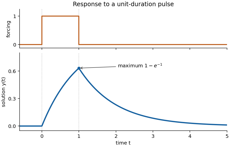
Codex 0 2026-10-14The forcing is a unit pulse on . For , the homogeneous equation and continuity with give . On , integration with gives . At the end of the pulse its value is , and the subsequent homogeneous decay must start at that value. ThusEquivalently it is the difference of two translated step responses, . The solution is continuous, rises concavely to its maximum at , and then decays exponentially to zero. Its derivative has jumps at the pulse edges; those are permitted because the right-hand side has step discontinuities.
Pinned article: Introduction to the OurBigBook Project
Welcome to the OurBigBook Project! Our goal is to create the perfect publishing platform for STEM subjects, and get university-level students to write the best free STEM tutorials ever.
Everyone is welcome to create an account and play with the site: ourbigbook.com/go/register. We belive that students themselves can write amazing tutorials, but teachers are welcome too. You can write about anything you want, it doesn't have to be STEM or even educational. Silly test content is very welcome and you won't be penalized in any way. Just keep it legal!
Intro to OurBigBook
. Source. We have two killer features:
- topics: topics group articles by different users with the same title, e.g. here is the topic for the "Fundamental Theorem of Calculus" ourbigbook.com/go/topic/fundamental-theorem-of-calculusArticles of different users are sorted by upvote within each article page. This feature is a bit like:
- a Wikipedia where each user can have their own version of each article
- a Q&A website like Stack Overflow, where multiple people can give their views on a given topic, and the best ones are sorted by upvote. Except you don't need to wait for someone to ask first, and any topic goes, no matter how narrow or broad
This feature makes it possible for readers to find better explanations of any topic created by other writers. And it allows writers to create an explanation in a place that readers might actually find it.
Figure 1. Screenshot of the "Derivative" topic page. View it live at: ourbigbook.com/go/topic/derivativeVideo 2. OurBigBook Web topics demo. Source. - local editing: you can store all your personal knowledge base content locally in a plaintext markup format that can be edited locally and published either:This way you can be sure that even if OurBigBook.com were to go down one day (which we have no plans to do as it is quite cheap to host!), your content will still be perfectly readable as a static site.
- to OurBigBook.com to get awesome multi-user features like topics and likes
- as HTML files to a static website, which you can host yourself for free on many external providers like GitHub Pages, and remain in full control

Figure 2. You can publish local OurBigBook lightweight markup files to either OurBigBook.com or as a static website.
Figure 3. Visual Studio Code extension installation.
Figure 5. . You can also edit articles on the Web editor without installing anything locally. Video 3. Edit locally and publish demo. Source. This shows editing OurBigBook Markup and publishing it using the Visual Studio Code extension. 
- Infinitely deep tables of contents:




All our software is open source and hosted at: github.com/ourbigbook/ourbigbook
Further documentation can be found at: docs.ourbigbook.com
Feel free to reach our to us for any help or suggestions: docs.ourbigbook.com/#contact