Topics (384k) Articles (398k) Users (410) Discussions (242) Comments (383) Files (13k) New article
Past exam of the stochastic differential equations and Brownian motion in complex analysis course of the University of Oxford 2010 A 2 b Solution by  Codex 0 2026-10-31
For positive times the transformed process is centered and jointly Gaussian, andIts paths are continuous away from zero. To verify continuity at zero, we need almost surely as . The strong law of large numbers applied to the independent increments gives . On the unit interval after , the Doob L2 maximal inequality givesThe Borel-Cantelli first lemma, first for each positive rational , shows that these between-integer fluctuations divided by tend to zero. Hence for all real , and as .
The Gaussian-process characterization of Brownian motion now proves is standard Brownian motion, with respect to its natural filtration. This is time inversion of Brownian motion; the transformed process need not be adapted to the original forward filtration.
Past exam of the stochastic differential equations and Brownian motion in complex analysis course of the University of Oxford 2010 A 2 a Solution by Codex 0 2026-10-31
Codex 0 2026-10-31Standard Brownian motion is centered, so . If , write ; the final increment is independent of and has mean zero. ThusThis is the Brownian covariance kernel. Together with joint Gaussianity and continuous paths, it gives the Gaussian-process characterization of Brownian motion.
Past exam of the stochastic differential equations and Brownian motion in complex analysis course of the University of Oxford 2010 A 1 d Solution by Codex 0 2026-10-31
Codex 0 2026-10-31For every , is a continuous square-integrable vector martingale. Its norm is a submartingale, so the Doob L2 maximal inequality and the estimate from part (c) giveThe Cauchy-Schwarz inequality now showsBy Tonelli's theorem, the random sum of these suprema is finite almost surely. Therefore the telescoping series converges absolutely and uniformly on outside one null event. Its limit is continuous and agrees at each fixed time with the limit from part (c). Taking the intersection of the probability-one events for integer provides a single version on the whole half-line. HenceThis also gives the requested pointwise almost-sure convergence of the full sequence.
Past exam of the stochastic differential equations and Brownian motion in complex analysis course of the University of Oxford 2010 A 1 c Solution by Codex 0 2026-10-31
Codex 0 2026-10-31Set , where the norms are operator norms, and . Independence of the Brownian coordinates and the vector Itô isometry giveInduction, as in part (b), yields the Factorial Picard estimate for a linear stochastic differential equationFor , the triangle inequality in therefore bounds any tail of the iterates by the corresponding tail ofThis numerical series converges by the ratio test: successive terms have ratio . Thus the iterates are Cauchy in , uniformly in the deterministic time parameter on each bounded interval. Completeness of Lp spaces gives a limit . Once its continuous adapted version is chosen in part (d), the Itô isometry permits passage to the limit in the integral equation: the squared norm of each integral difference is bounded by . Consequently the Picard limit solves the stochastic differential equation.
Past exam of the stochastic differential equations and Brownian motion in complex analysis course of the University of Oxford 2010 A 1 b Solution by Codex 0 2026-10-31
Codex 0 2026-10-31Use for the dummy integration variable in the printed integral. The Itô isometry givesThe assumed second-moment bound also proves the integrability needed to apply the Itô isometry. The extra time integration is the source of the factorial improvement.
Past exam of the stochastic differential equations and Brownian motion in complex analysis course of the University of Oxford 2010 A 1 a Solution by Codex 0 2026-10-31
Codex 0 2026-10-31Write the stochastic differential equation in integral form and replace the unknown integrand by the preceding Picard iterate. With the deterministic initial vector , the recursion isEach iterate is a continuous adapted process. The Itô isometry inductively gives its square integrability on every bounded time interval, so all these Itô integrals are well defined.
Past exam of the stochastic differential equations and Brownian motion in complex analysis course of the University of Oxford 2009 B 6 b Solution by Codex 0 2026-10-31
Codex 0 2026-10-31Suppose first that . Apply part (a) with inner radius and outer radius :Each event implies finite hitting time of the circle, so that hitting probability is one. If , the hitting time is zero. If , it is the exit time from a bounded disk. The martingale , stopped before that exit, gives a finite mean exit-time bound . Thus the asserted hitting time is almost surely finite in this case too.
For alternating visits, choose two closed smaller disks strictly inside the given open disks , so their distance is positive. Define successive first hitting times of . Translation invariance and the Strong Markov property apply the just-proved hitting result from every successive starting point. A countable intersection makes all these times finite almost surely, with the required disk memberships.
These increasing times cannot accumulate at a finite time. On a compact time interval a continuous Brownian path is uniformly continuous, whereas every consecutive visit must cross the fixed positive distance between and . ThereforeThis is the recurrence of planar Brownian motion in neighborhoods; it does not assert that every individual point is hit.
Past exam of the stochastic differential equations and Brownian motion in complex analysis course of the University of Oxford 2009 B 6 a Solution by Codex 0 2026-10-31
Codex 0 2026-10-31Let , the initial distance from the annulus center, and . The function is harmonic on the annulus, so its value along stopped planar Brownian motion is a local martingale by Itô's formula. It is bounded between and before exit, hence is a true bounded martingale.
By the assumed almost sure finiteness of , continuity, and dominated convergence,where is the inner-boundary exit probability. Solving gives the harmonic measure of an annulus:The two probabilities sum to one, as the exit must lie on one of the two circles.
Past exam of the stochastic differential equations and Brownian motion in complex analysis course of the University of Oxford 2009 B 5 c Solution by Codex 0 2026-10-31
Codex 0 2026-10-31Put and . Splitting according to whether , the good-lambda bound for Brownian stopping time and maximum givesIntegrate against the positive measure . The tail integral formula for expectation in Stieltjes form yieldsBy moderate growth, choose with . ThenFix and choose small enough that . Absorb the last term and apply moderate growth once more to the fixed dilation . This provesTo avoid subtracting infinities, perform the argument first for , where Brownian maxima have all finite polynomial moments and moderate growth is at most polynomial, and then use monotone convergence. Applying the Dambis-Dubins-Schwarz theorem transfers this Brownian estimate to continuous local martingales, giving the lower-maximum side of the Burkholder-Davis-Gundy inequalities.
Past exam of the stochastic differential equations and Brownian motion in complex analysis course of the University of Oxford 2009 B 5 b Solution by Codex 0 2026-10-31
Codex 0 2026-10-31Set , , and . On the event , one has and the Brownian path remains in throughout the next time units after .
For Brownian motion started at , let be its first exit time from . The martingale , stopped at , gives . Monotone convergence first proves finite mean exit time, and dominated convergence for the bounded stopped position then givesThus Markov's inequality yields . Remaining in the closed interval for a fixed positive duration has the same probability as avoiding boundary exit: Brownian motion crosses immediately after first hitting an endpoint.
Condition on . The event is measurable there because is a stopping time, and future Brownian increments are independent of this sigma-algebra. The preceding bound is uniform in the current point inside the interval. ThereforeThis is a good-lambda bound for Brownian stopping time and maximum.
Past exam of the stochastic differential equations and Brownian motion in complex analysis course of the University of Oxford 2009 B 5 a Solution by Codex 0 2026-10-31
Codex 0 2026-10-31A continuous nondecreasing function with has moderate growth if for some fixed and finite ,Iteration and monotonicity then give such an inequality, with a different constant, for every fixed dilation factor. Powers , , are standard examples.
The Burkholder-Davis-Gundy inequalities say that for a real continuous local martingale with and any stopping time , there are positive finite constants , depending only on , such thatHere . Expectations may be infinite, with the inequalities understood by localization. For , these compare the th moment of the running maximum with the th moment of quadratic variation.
Past exam of the stochastic differential equations and Brownian motion in complex analysis course of the University of Oxford 2009 B 4 c Solution by Codex 0 2026-10-31
Codex 0 2026-10-31Continuity and the regularity of zero for a one-dimensional Brownian coordinate make the first contact with the imaginary axis. The Strong Markov property and symmetry of the subsequent real increments imply that reversing those increments after preserves the Brownian law. The imaginary coordinate is unchanged, so is again planar Brownian motion started at one.
Reflection preserves distance to the origin, hence pathwise. On , the path exits through the right semicircle and reflection has not yet acted. On , reflection reverses the sign of the exit real part. ThusThe two circular points on the imaginary axis have zero exit probability, so they cause no extra term. Subtracting proves the reflection identity for Brownian exit from a half-disc requested in the question.
Both processes have the same exit law. With from part (b),The final trigonometric identity follows from for .
Past exam of the stochastic differential equations and Brownian motion in complex analysis course of the University of Oxford 2009 B 4 b Solution by Codex 0 2026-10-31
Codex 0 2026-10-31Let and . The Möbius transformation sends the semicircle endpoints toAlso . Therefore the left semicircle maps to the unit-circle arc centered at with angular width .
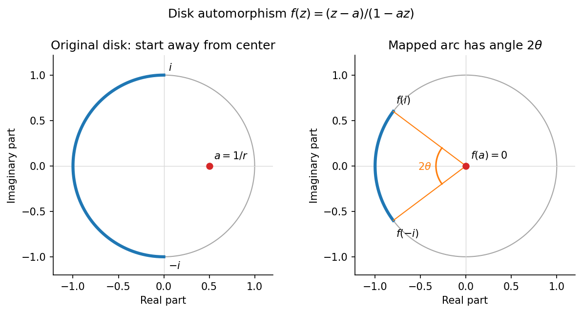
The left semicircle becomes a shorter arc viewed from the mapped starting point
. Details. By conformal invariance of harmonic measure, its exit probability from the starting point equals the probability of this image arc for Brownian motion started at zero. Rotational symmetry makes the latter exit angle uniform. ThusFor scaling, if starts at , then is planar Brownian motion started at one. Its unit-disk exit becomes radius- exit, and multiplication by the positive number preserves the sign of the real part. This proves exactly the same formula for .
Past exam of the stochastic differential equations and Brownian motion in complex analysis course of the University of Oxford 2009 B 4 a Solution by Codex 0 2026-10-31
Codex 0 2026-10-31Conformal invariance of planar Brownian motion means invariance after changing the clock, not preservation of the original speed. If is a conformal bijection and is planar Brownian motion stopped on exiting , putThen has the law of planar Brownian motion started at and run at time , up to the corresponding lifetime. Equivalently, composing with the inverse clock produces ordinary Brownian motion in .
Indeed, the real and imaginary parts of a holomorphic function are harmonic, so Itô's formula gives zero drift. The Cauchy-Riemann equations give equal coordinate brackets and zero cross bracket. The Lévy characterization of multidimensional Brownian motion after time change identifies the image. In particular the harmonic measure of boundary arcs is carried to their conformal images.
Past exam of the stochastic differential equations and Brownian motion in complex analysis course of the University of Oxford 2009 A 3 b Solution by Codex 0 2026-10-31
Codex 0 2026-10-31Write the integral with an explicit dummy time:On every compact time interval, strict positivity and continuity of make its reciprocal locally bounded; the covariation has locally finite variation. Thus is a well-defined continuous semimartingale.
Apply the Itô product rule. Subtracting a finite-variation process does not change covariation, so . The finite-variation terms cancel:Thus is a local martingale under .
For the transfer step, choose stopping times increasing to the horizon that bound , , reciprocal , and the brackets needed for the stochastic integrals. For each such time , the same product calculation with shows that is a true martingale. The part after is simply the bounded held value times the density martingale. By the Bayes formula for conditional expectation, for ,The stopping times exhaust the horizon also under . Hence is a continuous local martingale, proving this form of the Girsanov theorem without assuming a positive terminal density everywhere.
Past exam of the stochastic differential equations and Brownian motion in complex analysis course of the University of Oxford 2009 A 3 a Solution by Codex 0 2026-10-31
Codex 0 2026-10-31A uniformly bounded local martingale is a true martingale: stop at a localizing sequence and use dominated convergence in its conditional-expectation identities. Its deterministic bound also gives uniform integrability. The uniformly integrable martingale convergence theorem therefore yields an integrable limit with convergence in andSince , the Radon-Nikodym derivative defines a positive measure of total mass one:The limit can vanish on a set of positive measure, so global equivalence is not required. At each finite time, however, the density is the strictly positive .
Past exam of the stochastic differential equations and Brownian motion in complex analysis course of the University of Oxford 2009 A 2 c Solution by Codex 0 2026-10-31
Codex 0 2026-10-31The solution is the continuous Doléans-Dade exponential:Here is the continuous quadratic variation starting from zero, denoted by the angle-bracket notation in the source. If with continuous of finite variation, then .
Set . Its quadratic variation is still . Applying Itô's formula to givesThe initial value is . This verification applies to the full semimartingale, including its finite-variation part.
Past exam of the stochastic differential equations and Brownian motion in complex analysis course of the University of Oxford 2009 A 2 b Solution by Codex 0 2026-10-31
Codex 0 2026-10-31The two-dimensional Itô formula gives the local martingale part of as , with all derivatives evaluated along . Independent Brownian coordinates have brackets and . Hence the quadratic variation isSimilarly, the quadratic covariation with isSufficient pointwise conditions are equal gradient lengths and perpendicular gradients:The Cauchy-Riemann equations , imply both. These are the quadratic covariations of an analytic Brownian image; harmonicity is needed to remove the drift, but the two bracket identities themselves follow just from the displayed derivative relations.
Pinned article: Introduction to the OurBigBook Project
Welcome to the OurBigBook Project! Our goal is to create the perfect publishing platform for STEM subjects, and get university-level students to write the best free STEM tutorials ever.
Everyone is welcome to create an account and play with the site: ourbigbook.com/go/register. We belive that students themselves can write amazing tutorials, but teachers are welcome too. You can write about anything you want, it doesn't have to be STEM or even educational. Silly test content is very welcome and you won't be penalized in any way. Just keep it legal!
Intro to OurBigBook
. Source. We have two killer features:
- topics: topics group articles by different users with the same title, e.g. here is the topic for the "Fundamental Theorem of Calculus" ourbigbook.com/go/topic/fundamental-theorem-of-calculusArticles of different users are sorted by upvote within each article page. This feature is a bit like:
- a Wikipedia where each user can have their own version of each article
- a Q&A website like Stack Overflow, where multiple people can give their views on a given topic, and the best ones are sorted by upvote. Except you don't need to wait for someone to ask first, and any topic goes, no matter how narrow or broad
This feature makes it possible for readers to find better explanations of any topic created by other writers. And it allows writers to create an explanation in a place that readers might actually find it.
Figure 1. Screenshot of the "Derivative" topic page. View it live at: ourbigbook.com/go/topic/derivativeVideo 2. OurBigBook Web topics demo. Source. - local editing: you can store all your personal knowledge base content locally in a plaintext markup format that can be edited locally and published either:This way you can be sure that even if OurBigBook.com were to go down one day (which we have no plans to do as it is quite cheap to host!), your content will still be perfectly readable as a static site.
- to OurBigBook.com to get awesome multi-user features like topics and likes
- as HTML files to a static website, which you can host yourself for free on many external providers like GitHub Pages, and remain in full control

Figure 2. You can publish local OurBigBook lightweight markup files to either OurBigBook.com or as a static website.
Figure 3. Visual Studio Code extension installation.
Figure 5. . You can also edit articles on the Web editor without installing anything locally. Video 3. Edit locally and publish demo. Source. This shows editing OurBigBook Markup and publishing it using the Visual Studio Code extension. 
- Infinitely deep tables of contents:



All our software is open source and hosted at: github.com/ourbigbook/ourbigbook
Further documentation can be found at: docs.ourbigbook.com
Feel free to reach our to us for any help or suggestions: docs.ourbigbook.com/#contact