For fixed $n$, the likelihood ratio is strictly decreasing as $t^2$ increases. A likelihood-ratio test rejects for small $\lambda$, so its rejection rule is equivalently large $|t|$. Under the null hypothesis, the standard normal distribution and chi-squared distribution results give independent quantitiesTheir ratio therefore has Student's t-distribution with $n-1$ statistical degrees of freedom. The exact level-$\alpha$ rule isThis is precisely the two-sided Student's t-test; choosing the corresponding cutoff for $\lambda$ yields the same rejection region and the same p-value.

Define $R={\sum }_i(Y_i-\overline{Y}{)}^2$ and $s_Y^2=R/(n-1)$, with $n\ge 2$. The unrestricted maximum-likelihood estimates are $\hat{\mu }=\overline{Y}$ and ${\hat{\sigma }}^2=R/n$. Under the null hypothesis, maximizing the normal distribution's likelihood over the remaining variance givesbecause the cross term vanishes when ${\sum }_i(Y_i-\overline{Y})=0$. At either fitted variance, the exponential factor in the likelihood function is $e^{-n/2}$, so it cancels in the ratio:The standardized test statistic isThe sample variance $s_Y^2$ uses divisor $n-1$, whereas the maximum-likelihood estimate uses divisor $n$; this explains the $n-1$ in the final expression. Under a nondegenerate normal distribution, $R>0$ with probability one.

Here the exponential distribution is parametrized by its mean, so $f(x;\theta )={\theta }^{-1}{e}^{-x/\theta }$ for $x\ge 0$ and $\theta >0$. Its log-likelihood and maximum-likelihood estimate areFor one observation, ${\partial }_{\theta }\log f=-1/\theta +X/{\theta }^2$. Since $\mathrm{Var}(X)={\theta }^2$, its Fisher information is $I_1(\theta )=1/{\theta }^2$. Consequently the estimated standard error is $\overline{X}/\sqrt{n}$, givingThis is a large-sample confidence interval, not an exact one. If its lower endpoint is negative, intersecting with the parameter space $(0,\infty )$ removes impossible values without excluding any possible true statistical parameter.

Let $z={\Phi }^{-1}(1-\alpha /2)$, where $\Phi$ is the standard normal distribution's cumulative distribution function. Statistical consistency and Slutsky's theorem allow replacement of $I_1(\theta )$ by $I_1(\hat{\theta })$:Thus the probability that this standardized estimation error lies between $-z$ and $z$ tends to $1-\alpha$. Rearranging gives the Wald confidence intervalThe coverage probability is approximate, with limiting value $1-\alpha$; it is a repeated-sampling statement about the random confidence interval.

Write $I_1(\theta )$ for the Fisher information in one observation:Under the stipulated regularity assumptions, the maximum-likelihood estimator is consistent and has asymptotic normality:Equivalently, its large-sample normal approximation has mean $\theta$ and variance $1/[n{I}_1(\theta )]$. The information for the whole random sample is $n{I}_1(\theta )$; keeping the one-observation convention explicit prevents an extra factor of $n$.

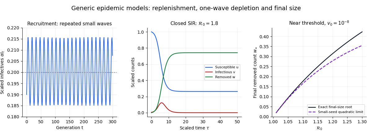
Divide the susceptible equation by the removed equation, or differentiate the resulting invariant directly, to get $du/dw=-{\mathcal{R}}_{0}u$. The initial data give the SIR susceptible-recovered identityPopulation conservation then gives $v=1+v_0-w-e^{-{\mathcal{R}}_{0}w}$. Since $w^{\prime }=v$, the Taylor expansion for small ${\mathcal{R}}_{0}w$ yieldsAt the end of the outbreak, the infectious count approaches zero. The positive root of the quadratic approximation isFor ${\mathcal{R}}_0>1$ and a seed satisfying ${\mathcal{R}}_0^2{v}_0\ll ({\mathcal{R}}_0-1{)}^2$, this reduces toThe truncation also requires ${\mathcal{R}}_0{w}_1\ll 1$, hence a near-threshold regime $0<{\mathcal{R}}_0-1\ll 1$. The seed must be small but positive: setting it identically to zero gives no epidemic. This is the near-threshold SIR final-size expansion, and the physical removed count is $S_0{w}_1$.

If the seed $v_0$ is positive, infection initially increases precisely whenIndeed, $v^{\prime }(0)=({\mathcal{R}}_0-1)v_0$. Susceptibility is nonincreasing, so if ${\mathcal{R}}_0\le 1$, the infectious count never starts an increasing phase. When ${\mathcal{R}}_0>1$, it grows until $u=1/{\mathcal{R}}_0$, the SIR infection peak, and then declines.

The basic reproduction number compares transmission and removal: one infectious individual generates infections at initial rate $\beta S_0$ and remains infectious for mean time $1/\gamma$. Their product $\beta S_0/\gamma$ is the expected number of secondary cases at that susceptible level. Above one, an infectious generation can replace itself with more cases. An exactly zero infectious seed remains zero regardless of this threshold.

Assume $S_0>0$ and scale by the initial susceptible count:Substitution into the SIR model equations givesThe initial data become $u(0)=1$, $v(0)=v_0$, $w(0)=0$. The conserved total is $u+v+w=1+v_0$, since the scaling is by $S_0$, not by $S_0+I_0$. With this normalization, ${\mathcal{R}}_0$ is the reproduction ratio at the initial susceptible level.

Yes, susceptible replenishment allows repeated outbreaks. While $I_t>0$, the infection ratio isInfection grows above the susceptible threshold $S_t=1/\alpha$ and declines below it. A wave depletes susceptibles; subsequent recruitment can restore the threshold and permit renewed growth. In the neutral linear regime, perturbations around the positive fixed point oscillate, so repeated small waves occur for sufficiently small perturbations over any fixed finite observation period.

For example, in scaled variables $x=\alpha S$, $y=\alpha I$, the choice $r=\alpha B=0.2$, $x_0=1.03$, $y_0=0.19$ produces the repeated positive waves illustrated below. This finite trajectory illustrates recurrence of outbreaks without claiming a nonlinearly attracting periodic orbit from the linearization alone. If $I_0=0$ exactly, the deterministic model has no infectious seed and $I_t$ stays zero.

At a fixed point the first equation gives $\alpha S_{\ast }{I}_{\ast }=B$. The second gives $I_{\ast }=\alpha S_{\ast }{I}_{\ast }$, so $I_{\ast }=B>0$ andThere is no disease-free fixed point: with $I=0$, susceptibles still increase by $B$ each step.

Set $r=\alpha B>0$. The Jacobian matrix of the update at the fixed point isIts characteristic equation and multipliers areFor $0<r<4$, these are distinct complex conjugates with product one, so both have modulus one. The linearized iterates are bounded and oscillatory: neutral linear stability holds for $0<\alpha B<4$, with no linear asymptotic attraction.

At $r=4$, the repeated multiplier is $-1$, but $M\ne -I$. Writing $M=-I+N$ gives $N\ne 0$, $N^2=0$ and $M^n=(-1{)}^n(I-nN)$, so generic linearized perturbations grow linearly. For $r>4$, a real multiplier has modulus greater than one. Thus the equilibrium is linearly unstable for $\alpha B\ge 4$.

For the unit-modulus range, the nonlinear behavior is not determined by this calculation: unit-modulus multipliers do not determine nonlinear stability.

The susceptible compartment retains $S_t$ individuals, gains $B$ recruits per generation and loses $\alpha S_t{I}_t$ through infection. The mass-action interaction term represents new infections generated by encounters between susceptible and infectious individuals. Those new cases form the next infectious compartment, $I_{t+1}$; the current infectious generation leaves that compartment after one time step.

The initial conditions $S_0,I_0$ specify the starting susceptible and infectious counts. The parameter $\alpha$ is the transmission coefficient in this deterministic approximation, while $B$ supplies new susceptible individuals. This is the discrete susceptible-infective model with recruitment.

For $R=(3/4)cT$, part (ii) requires ${\gamma }_B{v}_B/c\ge 3/4$, soThe speed formula in part (i) can be written $v_B/c=({\mathcal{E}}^2-m_B^2{c}^4)/({\mathcal{E}}^2+m_B^2{c}^4)$. Requiring it to be at least $3/5$ gives $\mathcal{E}\ge 2m_B{c}^2$, hence ${\gamma }_A{m}_A\ge m_B$.

Since ${\gamma }_A\ge 1$ already, the exact minimum isIn the second case, the rest energy of the incoming pair already suffices for the required outgoing speed. Keeping this mass-ratio case avoids taking the square root of a negative number.

The laboratory flight time is $R/v_B$. By time dilation, the accumulated proper time is $\tau =R/({\gamma }_B{v}_B)$. The definition of the rest-frame half-life gives at least one-half survival when $\tau \le T$, or ${\gamma }_B{v}_B\ge R/T$. Equivalently,Solving for the minimum speed givesUnder the usual exponential decay law, the survival probability is exactly $2^{-R/({\gamma }_B{v}_{B}T)}$. This is relativistic decay survival to a detector.

The two initial momenta cancel, so the laboratory is the centre-of-momentum frame. Let $\mathcal{E}=2{\gamma }_A{m}_A{c}^2$ be the total initial energy. Four-momentum conservation gives ${\mathbf{p}}_B=-{\mathbf{p}}_{\gamma }$ and $E_B+E_{\gamma }=\mathcal{E}$. The energy–momentum relation then yieldsThusUsing $v_B/c=c|{\mathbf{p}}_B|/E_B=E_{\gamma }/E_B$ givesThis is relativistic production of a massive particle and a photon. A positive-energy photon requires $\mathcal{E}>m_B{c}^2$; equality is the zero-photon-energy threshold.

The velocity vector is ${\mathbf{v}}_B=-v_B{\mathbf{n}}_{\gamma }$. Its direction is opposite the photon, but is not fixed relative to the incoming beam by conservation alone. Kinematics supplies its magnitude; an angular distribution needs the collision dynamics.

For a massless particle of energy $E>0$ moving in the unit direction $\mathbf{n}$,Its spatial momentum is $(E/c)\mathbf{n}$, and its four-momentum has Minkowski norm zero. A rest-frame expression $m\gamma (c,\mathbf{v})$ is not used for a massless particle.

Use the four-momentum convention $p^{\mu }=(E/c,\mathbf{p})$, with Minkowski signature $(+,-,-,-)$. For a particle of rest mass $m>0$ and three-velocity $\mathbf{v}$,Here $E=\gamma m{c}^2$ and $\mathbf{p}=\gamma m\mathbf{v}$, so $p^{\mu }{p}_{\mu }=m^2{c}^2$.

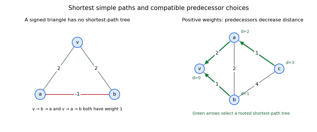
The unique root-to-$u$ path in $T$ is the reversal of its predecessor chain. Every edge satisfies $w(e_z)=d(z)-d(p(z))$. Summing along that chain telescopes tosince $d(v)=0$ for positive weights. Thus the tree path is a shortest $vu$-path in $G$ for every $u$, and $T$ is a shortest-path tree rooted at $v$.

Let $d(u)$ be the weight of a shortest $vu$-path, and let $p(u)$ be the predecessor of $u$ on the chosen $P_u$. Its prefix to $p(u)$ must also be shortest: a cheaper prefix followed by the final edge would give a cheaper walk to $u$, and cycle erasure in minimum-weight walks would produce a cheaper path because every edge weight is positive. ThereforeFollowing predecessor arrows strictly decreases $d$, so cannot revisit a vertex. Since each nonroot vertex has a predecessor, finiteness forces every predecessor chain to end at $v$. Thus $T$ is connected.

The edges $e_u$ are distinct: if two vertices selected the same undirected edge, each would be the other's predecessor, contradicting strict decrease. Hence $T$ has exactly $|V(G)|-1$ edges. A finite connected graph with this edge count is a tree. This proves that positive-weight shortest-path predecessors form a tree, without requiring the initially chosen paths to be mutually consistent.

A shortest-path tree rooted at $v$ is a spanning tree $T$ of $G$ for which the unique $vu$-path in $T$ is a $w$-shortest $vu$-path in $G$ for every vertex $u$. It simultaneously realizes all distances from the root. It need not be a minimum spanning tree, which minimizes total tree weight instead.

A shortest path from $u$ to $v$ is a graph path $P$ joining these endpoints such thatfor every other $uv$-path $P^{\prime }$ in $G$, where $w(P)$ is the sum of its edge weights. Here paths have no repeated vertices; minimizing over unrestricted walks is a different problem when negative edge weights occur.