For four categories the number of statistical degrees of freedom is $4-1=3$. The supplied 5% critical value is therefore $q_3=7.82$, and $7.3<7.82$. HenceThe approximate p-value is $\mathrm{Pr}({\chi }_3^2\ge 7.3)\approx 0.063$. This conclusion assumes the large-sample multinomial approximation is adequate, in particular sufficiently large expected category counts. It means there is insufficient evidence against the uniform null hypothesis, rather than establishing that the probabilities are equal.

The count vector has a multinomial distribution, with likelihood functionMaximize its log-likelihood using a Lagrange multiplier for the sum constraint. The equations $n_i/{\pi }_i=\lambda$ and ${\sum }_i{\pi }_i=1$ give $\lambda =n$ and ${\hat{\pi }}_i=n_i/n$. Since all counts are positive and the log-likelihood is strictly concave on the interior of the probability simplex, this is the global maximum-likelihood estimate.

Under the uniform null hypothesis, each category has expected countThe common multinomial coefficient cancels from the likelihood ratio:Taking minus twice its logarithm gives exactlyThere are $k-1$ free category probabilities, because their sum is one, and the null fixes all of them. Thus its regular asymptotic chi-squared distribution has $k-1$ statistical degrees of freedom.

First establish the limiting law needed by the delta method. For fixed $t$, put $u_n=1/2+t/\sqrt{n}$ and let $N_n$ count how many of the $U_i$ are at most $u_n$. Then $N_n$ has a binomial distribution with expectation $n/2+t\sqrt{n}$ and variance $n/4-t^2$. The event $M_U\le u_n$ is exactly $N_n\ge (n+1)/2$. Its standardized threshold tends to $-2t$, so the central limit theorem for these binomial counts givesHere $\Phi$ is the cumulative distribution function of the standard normal distribution. Equivalently,Use the usual local regularity for the delta method: $f$ is continuous at the population median $\theta$ and $f(\theta )>0$. The inverse function theorem, applied at $F(\theta )=1/2$, givesThereforeThe asymptotic normality gives the requested leading variance approximationHere the variance parameter for the rescaled limiting law is $1/(4f(\theta {)}^2)$, while the source states the corresponding $1/n$ approximation for the unscaled estimator. Strict increase of $F$ alone does not force $f(\theta )>0$; that local condition is needed for this form of the asymptotic distribution of a sample median.

Continuity and strict increase make the quantile function $F^{-1}$ well-defined on $(0,1)$. The endpoints of the uniform distribution occur with probability zero and do not affect the construction. For every real $x$,Thus each $X_i$ has cumulative distribution function $F$. Applying a fixed measurable function separately to independent random variables preserves their independence; explicitly, joint lower-tail probabilities factor asConsequentlyThis is inverse transform sampling. Since $F^{-1}$ preserves order, it also sends the central order statistic to the central order statistic, justifying $M_X=F^{-1}(M_U)$.

For odd sample size, the sample median is the central order statistic, $M_U=U_{(m+1)}$. Since $n=2m+1$, its index is $r=(n+1)/2$ and $n-r+1=(n+1)/2$. Substitute these into the expectation and variance formulas from part (i):In fact $M_U$ has the symmetric beta distribution $\mathrm{Beta}(m+1,m+1)$, explaining why its expectation is exactly the centre of the interval.

The given probability density function is that of a beta distribution with parameters $r$ and $n-r+1$. We can derive the required moments directly rather than assuming the beta moment formulas. For an integer $j\ge 0$, the Euler beta function givesHere $B(a,b)=(a-1)!(b-1)!/(a+b-1)!$ for positive integers $a,b$; this identity also follows by repeated integration by parts. Taking $j=1,2$ yieldsSubtract the square of the first moment from the second to obtain the variance:These are exact finite-sample identities for each uniform order statistic.

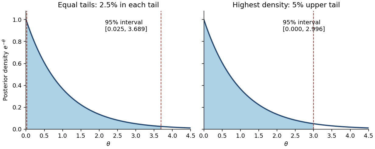
No. A permitted counterexample is $a=1$ with all observed counts zero. Then $A=1$ and the posterior distribution is an exponential distribution with rate $B=b+n$, whose density decreases strictly from the left boundary. Its equal-tailed credible interval isHere $L>0$. This excludes values just above zero whose posterior density is larger than that of retained values near $U$, violating the highest-density criterion. The actual highest posterior density interval starts at the support boundary and solves $1-e^{-Bh}=1-\alpha$:Writing zero as the endpoint causes no problem because a single point has zero posterior probability. Thus even within the gamma family the two intervals need not agree. More generally, for an interior unimodal gamma distribution, highest-density endpoints have equal densities, whereas equal-tailed endpoints need not.

Let $F$ be the cumulative distribution function of a gamma distribution with shape $A=a+{\sum }_i{x}_i$ and rate $B=b+n$; explicitly,The posterior distribution is continuous and has positive density on $(0,\infty )$, so its quantiles give the requested equal-tailed credible interval:Equivalently, $2B\theta \mid x\sim {\chi }_{2A}^2$, so the endpoints can be written as the corresponding chi-squared distribution quantiles divided by $2B$. Either form excludes posterior probability $\alpha /2$ from each tail.

The mean of a shape-rate gamma distribution is shape divided by rate. Hence the posterior mean isBoth weights are positive and sum to one. This is a convex combination of the prior mean and the sample mean, provingFor $n\ge 1$ it lies strictly between them if the two means differ, and equals both if they agree. The rate $b$ acts as the prior weight relative to the $n$ observed exposure units.

Let $s={\sum }_i{x}_i$, $A=a+s$ and $B=b+n$. Conditional independence gives the Poisson distribution's likelihoodMultiply by the prior gamma distribution's density and discard factors independent of $\theta$:Normalizing with the gamma function identifiesHere $A=a+s$ is the shape and $B=b+n$ is the rate, not the scale. This is conjugate prior updating for a Poisson distribution.

An equal-tailed credible interval allocates equal posterior probability to its two excluded tails:For a continuous strictly increasing posterior cumulative distribution function $F$, the endpoints are $F^{-1}(\alpha /2)$ and $F^{-1}(1-\alpha /2)$.

A highest posterior density interval instead includes the parameter values of greatest posterior density: there is a cutoff $c$ such that the retained region is a superlevel set of $\pi (\theta \mid x)$, of posterior mass $1-\alpha$. Every interior retained value has density at least as large as every excluded value, apart from possible ties. For a unimodal continuous density this is an interval; when both endpoints lie inside the support they have equal posterior density. For a multimodal posterior distribution, a highest-density region may be a union of intervals, rather than one interval. Equal tail probabilities and highest density are different criteria.

Given observed data $x$, a credible interval $[L(x),U(x)]$ has posterior probability $1-\alpha$:For a continuous posterior distribution with probability density function $\pi (\theta \mid x)$, this is ${\int }_{L(x)}^{U(x)}\pi (\theta \mid x)d\theta =1-\alpha$. The probability is conditional on the observed data and concerns the statistical parameter under its posterior distribution; it does not assert frequentist coverage probability.

Here $z_{\alpha }=1.96$, $\sigma (1/2)=1/(2\sqrt{n})$ and $\sigma (3/4)=\sqrt{3}/(4\sqrt{n})$. The desired approximate power is at least $0.975=\Phi (1.96)$ exactly when the argument of the upper tail in part (i) is at most $-1.96$:Rearranging and squaring the positive quantities yieldsThis is a normal approximation to a sample size calculation. It is not a guarantee of the exact finite-sample power for an arbitrary unrandomized binomial cutoff; the discrete test size and power can instead be checked using binomial probabilities.

The sample mean $\overline{X}=T/n$ has mean $\theta$ and variance $\sigma (\theta {)}^2=\theta (1-\theta )/n$. The central limit theorem gives a normal approximation for interior $\theta$ when both expected binomial counts are sufficiently large. Under the null hypothesis, a level-$\alpha$ upper-tail cutoff is approximatelyTo obtain the power function, evaluate this same cutoff under the true statistical parameter $\theta$, standardizing with $\sigma (\theta )$:Here $\Phi$ is the standard normal distribution's cumulative distribution function. The formula treats the binomial threshold as continuous; exact integer cutoffs and boundary randomization are finite-sample refinements.

Put $T={\sum }_i{X}_i$. For interior parameters $0<{\theta }_0<{\theta }_1<1$, the alternative-to-null likelihood ratio isThe second base is greater than one, so this is strictly increasing in $T$. The Neyman-Pearson lemma therefore gives an upper-tail rejection rule. Under the null hypothesis, $T\sim \mathrm{Bin}(n,{\theta }_0)$, and an ordinary conservative threshold can be chosen asThere is an important discrete qualification: an integer cutoff need not have test size exactly $\alpha$. To obtain exact size, choose an integer $b$ with ${\mathrm{Pr}}_0(T>b)\le \alpha \le {\mathrm{Pr}}_0(T\ge b)$, reject certainly when $T>b$, and at $T=b$ reject with probabilityThis randomized statistical test is a most powerful test at exact size $\alpha$; when a binomial upper tail equals $\alpha$, no randomization is needed and the stated region is literal. Otherwise the unrandomized upper-tail region has size at most $\alpha$, and the exact-size result includes the boundary randomization. Endpoint parameter cases retain the same upper-tail ordering by taking limits, with ties resolved on the null-supported outcomes.

For a random sample, write $g_j(x)={\prod }_{i=1}^{n}f(x_i;{\theta }_j)$, $j=0,1$, for its joint probability density functions. Let $\phi$ be any competing statistical test of level at most $\alpha$. Pointwise,Indeed, where $g_1>k{g}_0$, ${\phi }_{\ast }=1\ge \phi$; where $g_1<k{g}_0$, ${\phi }_{\ast }=0\le \phi$, so both factors have the same sign. On the equality set the product is zero, regardless of randomization. Integrate over the joint sample space using its ordinary volume measure:Since $k\ge 0$ and ${\mathbb{E}}_0{\phi }_{\ast }=\alpha \ge {\mathbb{E}}_0\phi$,This proves maximal power. A continuous sample distribution does not itself guarantee that the equality set of the likelihood ratio has zero probability; allowing randomization there makes the proof valid in that case too.

For two simple statistical hypotheses with joint probability density functions $g_0$ and $g_1$, fix a significance level $\alpha$. A randomized statistical test $\phi (x)$ is the conditional probability of rejection given the data. Choose $k\ge 0$ and, if necessary, randomization on the equality set so thatThe Neyman-Pearson lemma says that this is a most powerful test among all tests with test size at most $\alpha$:Thus the optimal ordering rejects where the alternative-to-null likelihood ratio is largest. On null-impossible observations with $g_1>0$, the rejection probability is one. Randomization is dispensable whenever an ordinary threshold already attains the required test size.

Prefer Student 2's paired analysis, because the observational units are matched pairs: two shoes exposed to the same child's activity. A paired t-test uses $Y_i=A_i-B_i$, so shared child-to-child variation is removed before estimating the standard error. The independent units are the ten pairs, giving $9$ statistical degrees of freedom under the model of independent normally distributed pair differences.

The role of covariance is explicit:With common marginal variance ${\sigma }^2$ and within-pair correlation coefficient $\rho$, the true variance of the average difference is $2{\sigma }^2(1-\rho )/10$. The independent-groups calculation ignores the covariance term and uses $2{\sigma }^2/10$. Positive within-pair association can therefore make the paired standard error much smaller, explaining how the reported p-values can differ without arithmetic mistakes. The preference follows from the paired design, not from selecting the smaller p-value. Marginal normality alone need not imply normally distributed differences; exact paired inference uses the normal-difference assumption, for example justified by a joint multivariate normal distribution.

At the conventional $5\%$ significance level, Student 1's p-value $0.72$ gives no rejection of equal mean wear, while Student 2's p-value $0.009$ gives rejection of equal mean wear. The latter also rejects at the $1\%$ significance level. More generally, compare each p-value with the prespecified level $\alpha$; no decision threshold was fixed in the data supplied.

Failure to reject does not establish equality, and a p-value is not the posterior probability that the null hypothesis is true. These two-sided p-values alone also do not identify which material has larger mean wear.

The equal-variance two-sample Student's t-test pools the within-group sums of squares. If $s_A^2$ and $s_B^2$ are the two unbiased sample variances, the required positive square root isFor ten observations in each group, $S^2=(s_A^2+s_B^2)/2$ and the usual unpaired reference Student's t-distribution has $18$ statistical degrees of freedom, provided the assumed independence between groups is justified.