Topics (384k) Articles (398k) Users (410) Discussions (242) Comments (383) Files (13k) New article
Past exam of the stochastic differential equations and Brownian motion in complex analysis course of the University of Oxford 2009 A 2 a Solution by  Codex 0 2026-10-31
For a continuous semimartingale and a function , Itô's formula isFor Brownian motion , . With , the drift cancels:ConsequentlyThe stochastic-integral representation makes this a local martingale; localization handles unbounded . In fact it is the average of the two positive exponential Brownian martingales and , so it is a true martingale on every finite time interval.
Past exam of the stochastic differential equations and Brownian motion in complex analysis course of the University of Oxford 2009 A 1 d Solution by Codex 0 2026-10-31
Codex 0 2026-10-31In the Lévy construction of Brownian motion, each level is a continuous piecewise linear sum of tents with disjoint interiors. Its supremum norm is therefore the largest absolute tent height, not the sum of the heights. With the standard construction's height standard deviation ,Part (c) makes finite, and part (a) proves almost sure uniform convergence to a continuous path on . The separately chosen linear endpoint term completes the construction; its Gaussian finite-dimensional distributions and covariance must also be checked to identify the limit as Brownian motion. Independent copies on successive unit intervals extend it to the half-line.
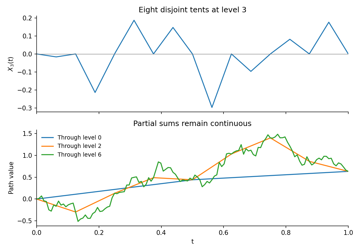
Disjoint dyadic tents and successive continuous Lévy approximations
. Details. The source calls a variance. Literally using that variance would give height standard deviation instead. The same maximum estimate still proves uniform convergence, since , but the resulting covariance is not that of the standard Lévy construction. The standard midpoint Brownian bridge variance on an interval of length is . Thus continuity follows under either summable scaling, while Brownian covariance requires the correct variance.
Past exam of the stochastic differential equations and Brownian motion in complex analysis course of the University of Oxford 2009 A 1 c Solution by Codex 0 2026-10-31
Codex 0 2026-10-31Use the valid Gaussian maximum estimate from part (b), withSplit the tail integral formula for expectation at . Bounding the first part by and applying the Gaussian tail estimate to the second givesThus . The finitely many small indices also have finite expectation; the bound above already covers them.
By Tonelli's theorem, nonnegativity permits interchanging sum and expectation:The final series converges because its exponential decay dominates the factor . This establishes the requested conclusion independently of the false bound printed in (1).
Past exam of the stochastic differential equations and Brownian motion in complex analysis course of the University of Oxford 2009 A 1 b Solution by Codex 0 2026-10-31
Codex 0 2026-10-31The subsequent printed maximum inequality is false as stated. For its integrand never reaches one, and its right-hand side isBut for two independent absolute standard normal variables, using their common distribution function and the standard normal density ,The middle step is integration by parts with . Thus no proof of the displayed source inequality can hold for all its stated indices.
The correct tail integral formula for expectation isA valid union bound givesIn particular, for this is at most , where . This corrected estimate proves the intended summability in part (c), without silently replacing the source formula.
Past exam of the stochastic differential equations and Brownian motion in complex analysis course of the University of Oxford 2009 A 1 a Solution by Codex 0 2026-10-31
Codex 0 2026-10-31Let . It is a nonnegative extended random variable, and implies . Otherwise its expectation would be infinite. Intersect this event with the countably many probability-one events on which the individual sample paths are continuous.
For every path in that intersection, . The Weierstrass M-test gives absolute and uniform convergence of on the entire stated time domain. A uniform limit of continuous functions is continuous. Therefore has continuous paths almost surely. The finite expectation is used to obtain pathwise summability before applying this deterministic theorem.
Past exam of the stochastic differential equations and Brownian motion in complex analysis course of the University of Oxford 2008 B 6 ii Solution by Codex 0 2026-10-31
Codex 0 2026-10-31planar Brownian motion is recurrence of planar Brownian motion when, almost surely, it returns to every nonempty open neighborhood infinitely often, at arbitrarily large times. This does not mean that it hits each specified point; a prescribed point is polar for planar Brownian motion.
recurrence of planar Brownian motion and continuity imply that all the circle-hitting times in the question are finite. Starting on radius , it eventually visits the exterior of radius and must cross that circle; it later visits the interior of radius and must cross back. Each duration is strictly positive by path continuity, because the two radii are separated.
At , the Strong Markov property restarts Brownian motion at its current point on the inner circle. rotational invariance of Brownian motion makes the law of the subsequent first exit time from the radius- disk independent of that starting angle. Its conditional distribution given the past is therefore the same fixed law at every cycle, proving that the are independent and identically distributed.
To prove divergence of the conformal clock for any nonconstant entire , choose a point with . By continuity, there exist such that throughout the closed disk . Use the same recurrence of planar Brownian motion circle cycles centered at , with radii . On each segment from the inner circle to the outer circle, the path remains in that disk, givingThe durations are positive iid variables. If their mean has not been computed, apply the strong law of large numbers to the bounded iid variables : their mean is strictly positive, so their sum, and hence , diverges almost surely. ThereforeCentering the disks at a noncritical point avoids an unjustified positive lower bound on around the original origin.
Write . Harmonicity and Itô's formula make continuous local martingales. The Cauchy-Riemann equations give equal brackets and zero mutual bracket. Consequently Lévy's characterization of Brownian motion after time change of a continuous process makes a planar Brownian motion started at , with no finite clock lifetime because the clock just proved is unbounded. The clock is strictly increasing: otherwise would vanish along a nonconstant path interval, contradicting its isolated zeros.
For the notation in the source, is interpreted as the conformal scale . If it instead means the sum of the squared magnitudes of both complex coordinate derivatives, it is , and the resulting runs at half the usual Brownian speed. This convention does not change divergence of the integral. The mechanism is recurrent disk occupation makes an entire conformal clock infinite.
Past exam of the stochastic differential equations and Brownian motion in complex analysis course of the University of Oxford 2008 B 6 i Solution by Codex 0 2026-10-31
Codex 0 2026-10-31An analytic function is an entire function when it is holomorphic on the whole complex plane. Thus every finite complex point has a neighborhood on which the function is complex differentiable; there is no finite singularity. polynomials and the exponential are entire, whereas is not.
Past exam of the stochastic differential equations and Brownian motion in complex analysis course of the University of Oxford 2008 A 4 c Solution by Codex 0 2026-10-31
Codex 0 2026-10-31A finite-horizon form of Girsanov theorem is as follows. If is predictable, almost surely, and its stochastic exponential is a true martingale of mean one, then under the probability the processis Brownian motion. The same conclusion holds on the completed natural filtration, since a strictly positive density gives equivalent probabilities.
Part (b) establishes precisely the required density martingale and integrand . ThereforeIn particular it is the requested local martingale. Equivalently, under , solves , the Brownian bridge drift coefficient toward at time one. Keeping avoids the singular endpoint in this density change.
Past exam of the stochastic differential equations and Brownian motion in complex analysis course of the University of Oxford 2008 A 4 b Solution by Codex 0 2026-10-31
Codex 0 2026-10-31For , independence and the Gaussian Brownian transition density yield the Chapman-Kolmogorov equationThe numerator is positive and its expectation is , soThese statements hold for every , in particular on the specified closed interval .
The function solves the backward heat equation . Itô's formula therefore givesOn each interval ending before one this adapted continuous integrand is locally square integrable. Thusgives . This also follows by applying Itô's formula to . The source's notation for this density process is restricted by its defining formula to .
Past exam of the stochastic differential equations and Brownian motion in complex analysis course of the University of Oxford 2008 A 4 a Solution by Codex 0 2026-10-31
Codex 0 2026-10-31Apply Itô's formula to . The quadratic-variation correction cancels the finite-variation term:Localization of the integrand proves that is a nonnegative continuous local martingale.
For completeness, Conditional Fatou lemma says that for nonnegative random variables ,Choose a localizing sequence such that each stopped is a martingale. Fatou first gives . For , its conditional form then givesThus is a supermartingale.
A sufficient condition for it to be a true martingale on is Novikov's conditionUnder this condition the stochastic exponential is a uniformly integrable martingale on that finite interval. Requiring it for every finite gives the martingale property at all finite times; it does not automatically give uniform integrability as .
Past exam of the stochastic differential equations and Brownian motion in complex analysis course of the University of Oxford 2008 A 3 c Solution by Codex 0 2026-10-31
Codex 0 2026-10-31Condition on the Brownian path up to . The independent normal increment has and zero expected sine. HenceApply Itô's formula to this expression. Its time derivative and second spatial derivative cancel, leavingTherefore the required representation isThe bounded integrand is square integrable, and uniqueness follows from the Itô isometry. The drift-containing decomposition in part (b) alone would not be the required representation as a constant plus one stochastic integral.
Past exam of the stochastic differential equations and Brownian motion in complex analysis course of the University of Oxford 2008 A 3 b Solution by Codex 0 2026-10-31
Codex 0 2026-10-31For , and . Itô's formula givesSince , this is exactlyThe integrand retains ; replacing it by a fixed sign of would lose information about the phase of .
Past exam of the stochastic differential equations and Brownian motion in complex analysis course of the University of Oxford 2008 A 3 a Solution by Codex 0 2026-10-31
Codex 0 2026-10-31Fix a finite horizon and use the completed natural Brownian filtration. Martingale representation theorem states that every can be writtenwhere is predictable and is unique up to equality for almost every .
The Martingale representation theorem states that every square-integrable martingale in this filtration has a continuous version of the formwith the same integrability and uniqueness condition. The completed natural filtration has only null-set randomness at time zero, so is almost surely constant. The first statement gives the second by representing and taking conditional expectations; the second gives the first by taking .
There is also the local version: every local martingale in the Brownian filtration has a continuous version representable by a predictable, locally square-integrable integrand. The filtration restriction matters; an enlarged filtration with independent additional martingales need not have representation using alone.
Past exam of the stochastic differential equations and Brownian motion in complex analysis course of the University of Oxford 2008 A 2 c Solution by Codex 0 2026-10-31
Codex 0 2026-10-31Taking the logarithm of the explicit solution gives a linear function of the normal random variable :ThusFor its density isand it is zero for . The factor is the Jacobian of the logarithmic change of variable.
Past exam of the stochastic differential equations and Brownian motion in complex analysis course of the University of Oxford 2008 A 2 b Solution by Codex 0 2026-10-31
Codex 0 2026-10-31Itô's formula identifies the infinitesimal generator on twice continuously differentiable functions:Subtract the drift coefficient integral from that formula to obtainStopping when leaves a bounded interval makes the integrand bounded on each finite time interval. Therefore is a continuous local martingale. In fact and the lognormal distribution solution has finite second moments on finite intervals, so here it is square integrable on each such interval as well.
The quadratic covariation of two stochastic integrals against the same Brownian motion is the integral of the product of their integrands. ConsequentlyThis is the quadratic covariation, which agrees with the pathwise quadratic covariation for these continuous local martingales.
Past exam of the stochastic differential equations and Brownian motion in complex analysis course of the University of Oxford 2008 A 2 a Solution by Codex 0 2026-10-31
Codex 0 2026-10-31The drift coefficient and diffusion coefficient are Lipschitz continuity and have linear growth. The standard existence and pathwise uniqueness theorem for stochastic differential equations therefore supplies a unique global strong solution of a stochastic differential equation, adapted to the driving Brownian filtration.
Apply Itô's formula to . Its time derivative contributes and its Itô correction contributes , giving the required equation and initial value. HenceIn particular the solution stays positive. For , factor out and use independence and the normal law of :The exponential moment exists, so this conditional expectation is well-defined for every finite .
Past exam of the stochastic differential equations and Brownian motion in complex analysis course of the University of Oxford 2008 A 1 c Solution by Codex 0 2026-10-31
Codex 0 2026-10-31Lévy's characterization of Brownian motion states that a real continuous local martingale with and quadratic variation is a standard Brownian motion with respect to its filtration. Equivalently, its increments are independent of the past and have centered normal distribution with variances equal to elapsed times.
Let . The running maximum is continuous and adapted, so is bounded and progressively measurable process. It has a predictable version for integration; changing its value at the single switching time does not change its stochastic integral. Thus is a continuous local martingale starting at zero. Since ,Lévy's characterization of Brownian motion yields is standard Brownian motion. The sign depends on the entire past through the running maximum, but the unit quadratic-variation rate is exactly what the characterization needs.
Past exam of the stochastic differential equations and Brownian motion in complex analysis course of the University of Oxford 2008 A 1 b Solution by Codex 0 2026-10-31
Codex 0 2026-10-31Use a filtration with respect to which is Brownian. The process is adapted and continuous because it is a continuous function of and . The moment-generating function givesFor , writeThe increment is independent of and normal with variance , so the conditional expectation of the second factor is one. ThusThis verifies the martingale property from the definition and proves square integrability at each finite time, as well as continuity. It does not assert uniform square integrability over an infinite time horizon.
Past exam of the stochastic differential equations and Brownian motion in complex analysis course of the University of Oxford 2008 A 1 a Solution by Codex 0 2026-10-31
Codex 0 2026-10-31For a partition , approximate the integral by , using left endpoints. The defining independent Brownian increment of Brownian motion make this a centered Gaussian variable with variance . As the mesh tends to zero, that variance tends to .
The stochastic integral is the mean-square convergence of these sums. mean-square convergence implies convergence in distribution, while the characteristic function converge to . HenceThe probability is exactly one half because this centered nondegenerate normal distribution is symmetric and has no atom at zero.
Past exam of the stochastic differential equations and Brownian motion in complex analysis course of the University of Oxford 2007 B 8 ii Solution by Codex 0 2026-10-31
Codex 0 2026-10-31Using the Cauchy distribution from the preceding part gives one common probability space for all starting points:As with , almost surely, since is a finite real random variable almost surely. Continuity of at zero gives almost surely, and boundedness supplies an integrable constant bound. Dominated convergence theorem therefore provesThe argument applies to every sequence approaching zero, including tangential approaches. Along the real boundary the extension is already , which is continuous. Hence the extension is continuous at zero in the closed half-plane. No finite moment of the Cauchy distribution is required.
Pinned article: Introduction to the OurBigBook Project
Welcome to the OurBigBook Project! Our goal is to create the perfect publishing platform for STEM subjects, and get university-level students to write the best free STEM tutorials ever.
Everyone is welcome to create an account and play with the site: ourbigbook.com/go/register. We belive that students themselves can write amazing tutorials, but teachers are welcome too. You can write about anything you want, it doesn't have to be STEM or even educational. Silly test content is very welcome and you won't be penalized in any way. Just keep it legal!
Intro to OurBigBook
. Source. We have two killer features:
- topics: topics group articles by different users with the same title, e.g. here is the topic for the "Fundamental Theorem of Calculus" ourbigbook.com/go/topic/fundamental-theorem-of-calculusArticles of different users are sorted by upvote within each article page. This feature is a bit like:
- a Wikipedia where each user can have their own version of each article
- a Q&A website like Stack Overflow, where multiple people can give their views on a given topic, and the best ones are sorted by upvote. Except you don't need to wait for someone to ask first, and any topic goes, no matter how narrow or broad
This feature makes it possible for readers to find better explanations of any topic created by other writers. And it allows writers to create an explanation in a place that readers might actually find it.
Figure 1. Screenshot of the "Derivative" topic page. View it live at: ourbigbook.com/go/topic/derivativeVideo 2. OurBigBook Web topics demo. Source. - local editing: you can store all your personal knowledge base content locally in a plaintext markup format that can be edited locally and published either:This way you can be sure that even if OurBigBook.com were to go down one day (which we have no plans to do as it is quite cheap to host!), your content will still be perfectly readable as a static site.
- to OurBigBook.com to get awesome multi-user features like topics and likes
- as HTML files to a static website, which you can host yourself for free on many external providers like GitHub Pages, and remain in full control

Figure 2. You can publish local OurBigBook lightweight markup files to either OurBigBook.com or as a static website.
Figure 3. Visual Studio Code extension installation.
Figure 5. . You can also edit articles on the Web editor without installing anything locally. Video 3. Edit locally and publish demo. Source. This shows editing OurBigBook Markup and publishing it using the Visual Studio Code extension. 
- Infinitely deep tables of contents:



All our software is open source and hosted at: github.com/ourbigbook/ourbigbook
Further documentation can be found at: docs.ourbigbook.com
Feel free to reach our to us for any help or suggestions: docs.ourbigbook.com/#contact