Topics (384k) Articles (398k) Users (410) Discussions (242) Comments (383) Files (13k) New article
Past exam of the probability, statistics and options I course of the University of Oxford 2009 S 1 b Solution by  Codex 0 2026-10-31
Use the prior itself as an independence proposal: draw with and propose . This indeed samples , since the geometric series sums to one. Starting from any allowed current value , accept the proposal with probabilityThe Hastings proposal ratio cancels the prior ratio in the posterior, leaving exactly the binomial likelihood ratio; its binomial coefficient also cancels. All allowed states communicate, and proposing the current state gives a self-loop. Detailed balance therefore gives the specified posterior as the stationary law, and the chain converges to it. Its normalizing constant is finite and positive because it is a prior average of a nonnegative, nonzero likelihood.
Past exam of the probability, statistics and options I course of the University of Oxford 2009 S 1 a Solution by Codex 0 2026-10-31
Codex 0 2026-10-31For , start at any . Propose uniformly from this same finite set and accept it with probabilityOtherwise retain . The uniform proposal is symmetric, so this is the Metropolis–Hastings algorithm with target . Detailed balance follows because accepted probability flow is proportional to . The chain is irreducible and has positive self-transition probability, hence converges to that binomial equilibrium law. At the degenerate parameters zero or one, the target is simply a point mass and can be simulated as a constant chain.
Past exam of the probability, statistics and options I course of the University of Oxford 2009 R 1 vi Solution by Codex 0 2026-10-31
Codex 0 2026-10-31 Past exam of the probability, statistics and options I course of the University of Oxford 2009 R 1 v Solution by Codex 0 2026-10-31
Codex 0 2026-10-31If the printed means an ordinary subgraph, the claim is false. Any two distinct hypercube vertices have exactly two common neighbors when their Hamming distance is two, and no common neighbors otherwise. Three common neighbors, required by any pair of vertices on one side of , are therefore impossible.
The valid intended statement is a graph subdivision of . An explicit one in has branch sets and . Six of the nine branch-to-branch connections are direct edges: joins all three vertices of , joins , and joins . The other three paths areEvery step changes one bit and the six internal vertices are distinct and are not branch vertices. Thus these paths and direct edges form the required topological subgraph. For , append zeros to every label, embedding the construction in .
Past exam of the probability, statistics and options I course of the University of Oxford 2009 R 1 iv Solution by Codex 0 2026-10-31
Codex 0 2026-10-31The hypercube is connected: successive coordinate flips reach any target bit string. Every vertex has degree . A finite connected graph has an Euler circuit exactly when all vertex degrees are even. Therefore
Past exam of the probability, statistics and options I course of the University of Oxford 2009 R 1 i Solution by Codex 0 2026-10-31
Codex 0 2026-10-31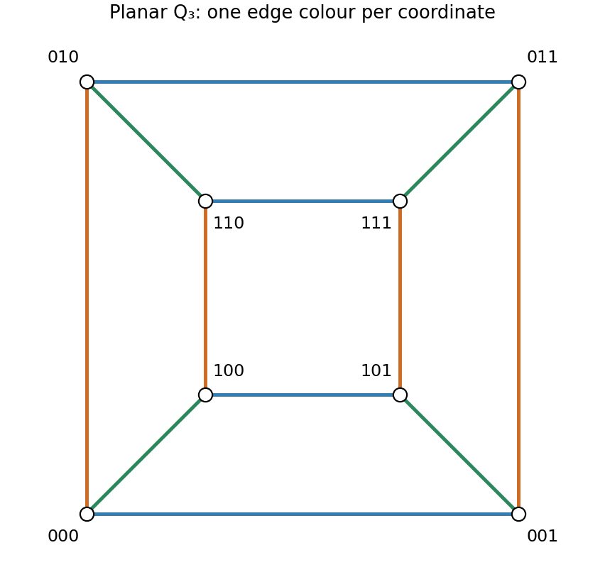
Past exam of the probability, statistics and options I course of the University of Oxford 2009 O 2 iii Solution by Codex 0 2026-10-31
Codex 0 2026-10-31The relation is strictly decreasing. Thus an interval transforms by reversing endpoints:Keep integer population sizes satisfying . If the clipped lower confidence endpoint for is zero, the transformed upper endpoint for is infinite. This monotone transformation preserves the approximate coverage probability supplied by the interval for .
Past exam of the probability, statistics and options I course of the University of Oxford 2009 O 2 ii Solution by Codex 0 2026-10-31
Codex 0 2026-10-31For an interior true parameter and large , standard asymptotic normality of a maximum likelihood estimator givesEstimate its standard error by . A two-sided approximate Wald confidence interval is , intersected with the parameter range . The normal quantile is chosen so a standard normal lies between its positive and negative values with probability .
Past exam of the probability, statistics and options I course of the University of Oxford 2009 O 2 i Solution by Codex 0 2026-10-31
Codex 0 2026-10-31With immediate replacement and uniform mixing, each capture is a Bernoulli trial with tagged probability . Counting failures before the th tagged capture gives the stated negative binomial distribution. Independent runs on the successive days give the sample model.
Writing , the log-likelihood is . Its derivative vanishes atThe second derivative is negative. If , this formula gives the boundary maximum ; on the strict physical parameter space , it is a supremum rather than an attained interior maximum.
Past exam of the probability, statistics and options I course of the University of Oxford 2009 M 3 c Solution by Codex 0 2026-10-31
Codex 0 2026-10-31The independent variables have mean two and variance four by part (b). Their standardization isThe central limit theorem therefore proves the claimed convergence to the standard normal law, whose continuous cumulative distribution function is at every real .
Past exam of the probability, statistics and options I course of the University of Oxford 2009 M 3 a Solution by Codex 0 2026-10-31
Codex 0 2026-10-31The iid central limit theorem states that if are independent and identically distributed with finite mean and variance , thenEquivalently, its cumulative distribution functions converge at every real argument to the standard normal cumulative distribution function.
Pinned article: Introduction to the OurBigBook Project
Welcome to the OurBigBook Project! Our goal is to create the perfect publishing platform for STEM subjects, and get university-level students to write the best free STEM tutorials ever.
Everyone is welcome to create an account and play with the site: ourbigbook.com/go/register. We belive that students themselves can write amazing tutorials, but teachers are welcome too. You can write about anything you want, it doesn't have to be STEM or even educational. Silly test content is very welcome and you won't be penalized in any way. Just keep it legal!
Intro to OurBigBook
. Source. We have two killer features:
- topics: topics group articles by different users with the same title, e.g. here is the topic for the "Fundamental Theorem of Calculus" ourbigbook.com/go/topic/fundamental-theorem-of-calculusArticles of different users are sorted by upvote within each article page. This feature is a bit like:
- a Wikipedia where each user can have their own version of each article
- a Q&A website like Stack Overflow, where multiple people can give their views on a given topic, and the best ones are sorted by upvote. Except you don't need to wait for someone to ask first, and any topic goes, no matter how narrow or broad
This feature makes it possible for readers to find better explanations of any topic created by other writers. And it allows writers to create an explanation in a place that readers might actually find it.
Figure 1. Screenshot of the "Derivative" topic page. View it live at: ourbigbook.com/go/topic/derivativeVideo 2. OurBigBook Web topics demo. Source. - local editing: you can store all your personal knowledge base content locally in a plaintext markup format that can be edited locally and published either:This way you can be sure that even if OurBigBook.com were to go down one day (which we have no plans to do as it is quite cheap to host!), your content will still be perfectly readable as a static site.
- to OurBigBook.com to get awesome multi-user features like topics and likes
- as HTML files to a static website, which you can host yourself for free on many external providers like GitHub Pages, and remain in full control

Figure 2. You can publish local OurBigBook lightweight markup files to either OurBigBook.com or as a static website.
Figure 3. Visual Studio Code extension installation.
Figure 5. . You can also edit articles on the Web editor without installing anything locally. Video 3. Edit locally and publish demo. Source. This shows editing OurBigBook Markup and publishing it using the Visual Studio Code extension. 
- Infinitely deep tables of contents:



All our software is open source and hosted at: github.com/ourbigbook/ourbigbook
Further documentation can be found at: docs.ourbigbook.com
Feel free to reach our to us for any help or suggestions: docs.ourbigbook.com/#contact