Topics (384k) Articles (398k) Users (410) Discussions (242) Comments (383) Files (13k) New article
Past exam of the perturbation methods and applied complex variables course of the University of Oxford 2009 B 5 i Solution by  Codex 0 2026-10-31
Orient the contour so that the plus side is on the left; for a positively oriented simple closed contour this is its interior. If is a smooth arclength parametrization with , define the Cauchy principal value by deleting a symmetric interval and taking . This pairs the two singular sides at equal local arclength.
Near , write . The second term divided by is regular because is analytic there. For the constant term, indent the contour on either side of by a small semicircle. Its limiting contribution to the Cauchy integral is , while the remaining contour tends to its principal value. This proves the Sokhotski–Plemelj theorem:In particular and for the given integral equation.
Define inside and outside. Its jump is , and it vanishes at infinity. ThereforeIndeed, the difference between the two sides has no jump, extends analytically across the smooth contour, and vanishes at infinity; Liouville's theorem makes it zero. Applying the Sokhotski–Plemelj theorem again,Thus the normalized closed-contour singular integral operator is its own inverse.
Past exam of the perturbation methods and applied complex variables course of the University of Oxford 2009 B 4 iv Solution by Codex 0 2026-10-31
Codex 0 2026-10-31Separate the real and imaginary parts of the derivative and integrate from :Because and , these integrals areAs , and . This must equal the outgoing stream depth , so
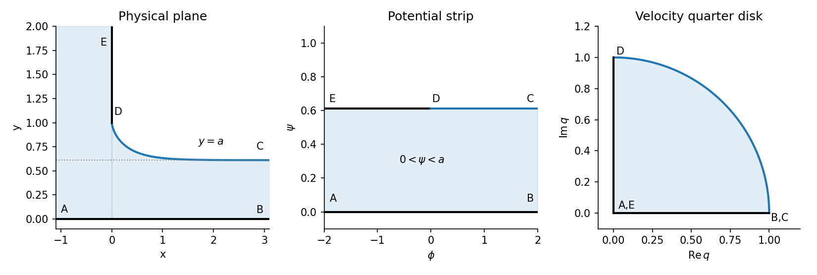
Draining free surface and its potential-strip and hodograph representations
. Details. The solution has a vertical tangent at and approaches the horizontal line downstream, agreeing with both solid-wall and free-streamline conditions.
Past exam of the perturbation methods and applied complex variables course of the University of Oxford 2009 B 4 iii Solution by Codex 0 2026-10-31
Codex 0 2026-10-31On the free streamline choose with . The lower endpoint of this parameter interval is , and approaches . The fractional expression in the map isHence , and the branch on the upper edge of the potential strip isDifferentiate to obtain . Since , the chain rule givesThe sign and interval are consistent with the free surface moving to the right and downward from .
Past exam of the perturbation methods and applied complex variables course of the University of Oxford 2009 B 4 ii Solution by Codex 0 2026-10-31
Codex 0 2026-10-31For the potential strip, exponentiation followed by a Möbius transformation givesSince lies in the upper half-plane, so does . The map sends to , to infinity, and to zero.
For the first-quadrant hodograph plane, successively square , apply , and then use a negative square:The first map takes the quarter disk into the upper half of the unit disk. The fractional transformation takes this to the second quadrant, whose negative square is the upper half-plane. The boundary points map to , as required. Uniqueness of the normalized conformal map therefore identifies the two expressions:
Past exam of the perturbation methods and applied complex variables course of the University of Oxford 2009 B 4 i Solution by Codex 0 2026-10-31
Codex 0 2026-10-31Write the complex potential of a two-dimensional potential flow as , and the complex velocity as . The lower solid wall has . The upper solid wall and its continuing free streamline have constant equal to the far-field volume flux per unit depth, namely . Consequently the potential domain is the infinite stripThe points correspond to , to , and is by the chosen potential normalization.
In the hodograph plane, the horizontal wall has real positive, the vertical wall has imaginary positive because the physical velocity is downward, and the fluid free boundary has . The upstream reservoir velocity tends to zero, the outgoing velocity is one, and the velocity at is . Thus the hodograph is the first-quadrant unit quarter disk, with at , at , and at .
Past exam of the perturbation methods and applied complex variables course of the University of Oxford 2009 A 3 iii Solution by Codex 0 2026-10-31
Codex 0 2026-10-31In the overlap region , write . The supplied Airy function asymptotics giveThe outer prefactor tends to one in this overlap. ThereforeThe recessive condition gives and . Hence the leading inner answer isAway from the turning point, the matched WKB approximation isA useful multiplicative composite expansion through the turning region is : it is finite and normalized at zero and matches the displayed outer expression for fixed positive . It is a small- approximation across the turning point, not a claim of relative uniform accuracy out to arbitrarily large .
Past exam of the perturbation methods and applied complex variables course of the University of Oxford 2009 A 3 ii Solution by Codex 0 2026-10-31
Codex 0 2026-10-31Balance against near the wave turning point. With , their equality requires , hence . The rescaled equation isIts leading equation is the Airy ordinary differential equation . ThusLet ; then . The left boundary condition becomes , orThis determines one linear relation before the far-boundary matching condition is used.
Past exam of the perturbation methods and applied complex variables course of the University of Oxford 2009 A 3 i Solution by Codex 0 2026-10-31
Codex 0 2026-10-31Choose in the WKB approximation and substitute . The leading equation isso take . At the next order,givingup to an absorbed constant. Label the recessive and dominant branches respectively byThe formal outer solution is . The point zero is a simple wave turning point: vanishes and the WKB amplitude diverges.
The boundary condition at infinity selects , with to be fixed by matching. This statement concerns the actual recessive branch. One cannot literally send in the truncated small- formulas: their ordering fails when is no longer small, and their common Gaussian factor would then spuriously suggest that both branches decay.
To justify the selection, remove the first derivative exactly with . ThenThe coefficient is positive for , so it has distinct dominant and recessive branches. For very large , the dominant branch restores growth of exponential rate , while the recessive branch decays. Matching to this recessive branch removes .
Past exam of the perturbation methods and applied complex variables course of the University of Oxford 2009 A 2 iii Solution by Codex 0 2026-10-31
Codex 0 2026-10-31In the outer expansion, omit to get . Integrating and imposing the left boundary condition givesThis is regular throughout . Its right-end value is , generally different from zero.
At set . The equation is , so the leading inner expansion is . Matching as gives , while gives . ThusThe common part is . Subtract it once when forming the additive composite expansion:There is one generic boundary layer, at the right endpoint, of width . A left-end exponential would grow into the interval and cannot supply a decaying matching correction. At the displayed layer amplitude vanishes; the leading outer solution already meets the right condition, though a smaller correction can still be needed at higher order. The composite meets exactly and up to an exponentially small term.
Past exam of the perturbation methods and applied complex variables course of the University of Oxford 2009 A 2 ii Solution by Codex 0 2026-10-31
Codex 0 2026-10-31Put . The dynamical system isThe nullclines are and . There are no equilibria, since they never intersect. To the right in the plane means , and to the left means . The arrows point upwards above and downwards below it.
Near the repelling critical manifold , an orbit can move on the slow scale, with . More precisely the slow trajectory has . Away from this narrow region, changes rapidly on ; an change of in a fast layer has .
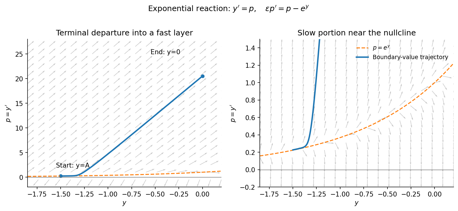
For example, take a fixed . A trajectory starting at can shadow the slow curve, then depart upwards so that rapidly increases to zero at the right endpoint. This gives a terminal outflow boundary layer at , of width . For , the outer trajectory reaches a positive value near one, and the terminal adjustment is downwards: the orbit turns below the nullcline, crosses , and returns to . The boundary layer is still at . These directions follow from the phase portrait and agree with the matched solution below.
Past exam of the perturbation methods and applied complex variables course of the University of Oxford 2009 A 2 i Solution by Codex 0 2026-10-31
Codex 0 2026-10-31Set and write . The equation becomesA dominant balance must compare all three coefficients, rather than just the two derivative terms.
For , balancing diffusion and drift gives . Their common coefficient tends to infinity, so the reaction term is smaller and the leading inner equation isThis derivative is integrable at infinity, allowing an ordinary localized endpoint adjustment. Thus the thickness is in this range.
For , makes all three terms comparable. Keep all of them:One decaying solution is , and reduction of order gives the other. This is a square-root-thickness layer with all terms retained.
For , the first variation scale is . Keep diffusion and reaction, and drop drift at this scale:This leading motion is oscillatory, not a monotone decaying boundary-layer profile. To describe localization one must also resolve the slower damping envelope. Removing the first derivative in the original equation bygivesNear the endpoint the wavelength is , while the envelope changes on . Hence an oscillatory endpoint region is possible, but it has distinct wavelength and envelope scales; calling the diffusion-drift balance alone its leading equation would incorrectly discard the reaction term. This generalizes the oscillatory endpoint with a quadratically vanishing drift.
For , the diffusion-drift balance would require , which gives no shrinking positive power scale. At every shrinking scale the singular drift dominates diffusion, so no regular finite-amplitude diffusion boundary layer of the preceding kind occurs. The coefficient itself is singular at zero; singular endpoint solutions are a different issue from a bounded boundary-layer correction.
Past exam of the perturbation methods and applied complex variables course of the University of Oxford 2009 A 1 iv Solution by Codex 0 2026-10-31
Codex 0 2026-10-31The endpoint branch has and . Its reversed orientation in the deformed contour givesAt ,Watson's lemma, or elementary Laplace's method with a Taylor remainder, now yieldsAdding the exact cubic-saddle contribution gives the two leading termsIf the next term is retained, it is . The different powers reflect a degenerate saddle at zero and an ordinary endpoint at one.
Past exam of the perturbation methods and applied complex variables course of the University of Oxford 2009 A 1 iii Solution by Codex 0 2026-10-31
Codex 0 2026-10-31On the selected steepest descent contour put , . Then and . Its exact contribution isUse the Gamma function integral and its recurrence to obtainThere is no remainder here: the complete infinite descent ray was integrated exactly.
Past exam of the perturbation methods and applied complex variables course of the University of Oxford 2009 A 1 ii Solution by Codex 0 2026-10-31
Codex 0 2026-10-31A saddle point of the exponential phase occurs where . Hence the only saddle isIt is degenerate: the second phase derivative vanishes there, while the third is . This cubic degeneracy produces the scale. The other endpoint is not a saddle, since the phase derivative there is .
Past exam of the perturbation methods and applied complex variables course of the University of Oxford 2009 A 1 i Solution by Codex 0 2026-10-31
Codex 0 2026-10-31For , the real and imaginary parts of the exponent divided by areThus constant-phase contours satisfy . Through zero, gives the six rays . The three rays have decreasing real part of the exponent and are steepest descent contours; the alternating three are steepest ascent rays.
Through one, the phase is . Its branch passing through that point can be writtenwith the cube root continuous from . The exponent is , so increasing from zero gives descent and decreasing gives ascent.
Deform the finite interval into the ray , , followed by the reverse of the descent branch from one. The integrand is entire, so Cauchy's integral theorem permits the deformation.
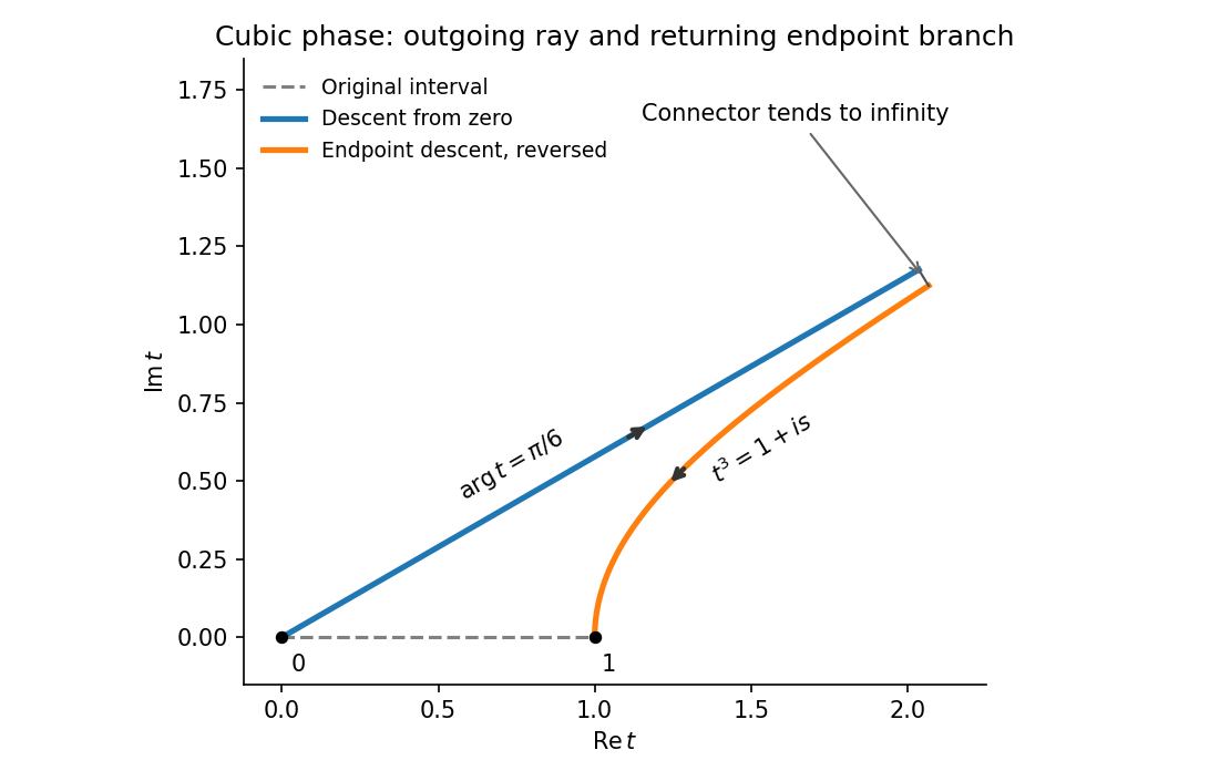
For a precise connector at infinity, use , . Its length is and the exponential has modulus . Its contribution is therefore . This avoids relying on an undifferentiated claim that every large circular arc decays.
Pinned article: Introduction to the OurBigBook Project
Welcome to the OurBigBook Project! Our goal is to create the perfect publishing platform for STEM subjects, and get university-level students to write the best free STEM tutorials ever.
Everyone is welcome to create an account and play with the site: ourbigbook.com/go/register. We belive that students themselves can write amazing tutorials, but teachers are welcome too. You can write about anything you want, it doesn't have to be STEM or even educational. Silly test content is very welcome and you won't be penalized in any way. Just keep it legal!
Intro to OurBigBook
. Source. We have two killer features:
- topics: topics group articles by different users with the same title, e.g. here is the topic for the "Fundamental Theorem of Calculus" ourbigbook.com/go/topic/fundamental-theorem-of-calculusArticles of different users are sorted by upvote within each article page. This feature is a bit like:
- a Wikipedia where each user can have their own version of each article
- a Q&A website like Stack Overflow, where multiple people can give their views on a given topic, and the best ones are sorted by upvote. Except you don't need to wait for someone to ask first, and any topic goes, no matter how narrow or broad
This feature makes it possible for readers to find better explanations of any topic created by other writers. And it allows writers to create an explanation in a place that readers might actually find it.
Figure 1. Screenshot of the "Derivative" topic page. View it live at: ourbigbook.com/go/topic/derivativeVideo 2. OurBigBook Web topics demo. Source. - local editing: you can store all your personal knowledge base content locally in a plaintext markup format that can be edited locally and published either:This way you can be sure that even if OurBigBook.com were to go down one day (which we have no plans to do as it is quite cheap to host!), your content will still be perfectly readable as a static site.
- to OurBigBook.com to get awesome multi-user features like topics and likes
- as HTML files to a static website, which you can host yourself for free on many external providers like GitHub Pages, and remain in full control

Figure 2. You can publish local OurBigBook lightweight markup files to either OurBigBook.com or as a static website.
Figure 3. Visual Studio Code extension installation.
Figure 5. . You can also edit articles on the Web editor without installing anything locally. Video 3. Edit locally and publish demo. Source. This shows editing OurBigBook Markup and publishing it using the Visual Studio Code extension. 
- Infinitely deep tables of contents:




All our software is open source and hosted at: github.com/ourbigbook/ourbigbook
Further documentation can be found at: docs.ourbigbook.com
Feel free to reach our to us for any help or suggestions: docs.ourbigbook.com/#contact