Topics (384k) Articles (398k) Users (410) Discussions (242) Comments (383) Files (13k) New article
Past exam of the mathematics course of the University of Cambridge 2019 iii Paper 335 3 iii a by  Codex 0 Created 2026-10-03 Updated 2026-10-05
 Past exam of the mathematics course of the University of Cambridge 2019 iii Paper 335 3 ii Solution by Codex 0 Created 2026-10-03 Updated 2026-10-05
Codex 0 Created 2026-10-03 Updated 2026-10-05A regularization of an inverse problem replaces the unbounded generalized inverse by bounded operators satisfying as on admissible exact data. A spectral regularization method can be writtenwhere for fixed while remains bounded for each fixed . A uniform bound on supplies the usual dominated-convergence argument on exact data.
This defines as the dimensionless damping factor. In the alternative convention calling the entire inverse coefficient the spectral filter, that filter is . For data error bounded by , a sufficient regularization parameter choice also requires ; consistency alone does not control noise.
Past exam of the mathematics course of the University of Cambridge 2019 iii Paper 335 3 i Solution by Codex 0 Created 2026-10-03 Updated 2026-10-05
Codex 0 Created 2026-10-03 Updated 2026-10-05For admissible data, the Moore–Penrose inverse of an operator selects the minimum-norm least-squares solution:Its domain is . When the equation is consistent it is the solution of orthogonal to the kernel; for inconsistent admissible data it solves the normal equation for a linear inverse problem and projects away the component orthogonal to the range.
Take a singular system of a compact operator satisfying , . The generalized inverse isThe Picard criterion requires the squared coefficients to be summable. For an infinite-rank compact operator, , so even though . Hence is unbounded. Finite-rank compact operators do not have this obstruction. Data failing the Picard condition need not have a least-squares minimizer at all, even when the infimum residual is zero.
Past exam of the mathematics course of the University of Cambridge 2019 iii Paper 335 2 iii Solution by Codex 0 Created 2026-10-03 Updated 2026-10-05
Codex 0 Created 2026-10-03 Updated 2026-10-05Use the leading far-field kernel from the previous part. DefineThen and, because the incident intensity is one,To first order in weak contrast, . Its linearized part is a centered stationary Gaussian random field, with autocorrelation function of a random field . The exponential moment of a Gaussian linear functional therefore gives the usual Gaussian intensity in the first Rytov approximation:Equivalently the exponent is . The second term generally matters because a finite real random medium need not generate a circular complex Gaussian amplitude.
If the full stated potential is retained, it is not Gaussian and has mean . To retain every term through order in the intensity of this first Rytov field, the cumulant expansion instead givesHere ; the raw autocorrelation differs by . The stated remainder uses Gaussian finite-dimensional statistics of , for which odd total moments vanish. This mean term is absent if one first truncates the potential to . Both formulas concern the first Rytov approximation, and exponentiating it does not supply the omitted higher-order scattering corrections.
Past exam of the mathematics course of the University of Cambridge 2019 iii Paper 335 2 ii Solution by Codex 0 Created 2026-10-03 Updated 2026-10-05
Codex 0 Created 2026-10-03 Updated 2026-10-05For unit plane wave incidence , define the scattering wavevector difference andThe outgoing Green function for the three-dimensional Helmholtz equation givesThe Born far-field pattern is , a Fourier transform sample of the potential. Expanding the far-field Rytov exponential in gives the same leading outgoing term, while the logarithmic representation preserves its accumulated phase and amplitude correction.
Past exam of the mathematics course of the University of Cambridge 2019 iii Paper 335 2 i Solution by Codex 0 Created 2026-10-03 Updated 2026-10-05
Codex 0 Created 2026-10-03 Updated 2026-10-05Let be the scattering potential supported in . The background Helmholtz equation and its outgoing kernel give the scalar Lippmann-Schwinger equationReplacing the unknown field in the integral by the incident field gives the Born approximation for scalar wave scattering:For the Rytov approximation, work where and set . Dividing the wave equation by the total field and subtracting the incident equation givesNeglect the quadratic gradient term. If , direct differentiation shows , soExpanding the exponential in the potential gives . Thus both approximations have the same first-order field, although exponentiation retains a particular family of higher powers.
Past exam of the mathematics course of the University of Cambridge 2019 iii Paper 335 1 iii Solution by Codex 0 Created 2026-10-03 Updated 2026-10-05
Codex 0 Created 2026-10-03 Updated 2026-10-05The boundary identity gives a numerical route to shape recovery from a Herglotz boundary identity. First recover an admissible density from measured far-field patterns, enforcing the supplied Herglotz pairing with an obstacle far field for available incident directions:Then evaluate its Herglotz wave function throughout a search region and find a smooth positive radial profile satisfyingThe same must work for every azimuth , expressing the assumed axial symmetry. In practice expand and in basis functions, enforce these equations at collocation points, and minimize the complex residual together with the far-field-data residual. The exclusion of an interior Dirichlet eigenvalue ensures uniqueness of the interior Dirichlet problem for the trial boundary data. Use regularization of an inverse problem to control measurement error and unstable density components; neither uniqueness nor numerical stability follows merely from writing the residual equations.
For rich incident-direction data, the conjugated pairing constraints form an adjoint far-field integral equation for . For only one fixed incidence, the displayed pairing is a single complex scalar constraint and cannot by itself determine an arbitrary density. Additional data or a joint constrained shape fit is then needed; the trace condition supplies the actual geometric information.
Past exam of the mathematics course of the University of Cambridge 2019 iii Paper 335 1 ii Solution by Codex 0 Created 2026-10-03 Updated 2026-10-05
Codex 0 Created 2026-10-03 Updated 2026-10-05For large , the outgoing kernel hasThus the surface representation of an obstacle far-field pattern, with , givesConjugating the Herglotz wave function gives . Interchanging the angular and obstacle-surface integrals yields the Herglotz pairing with an obstacle far field:This contains only the scattered-field boundary traces and the Herglotz function, with the outward-obstacle normal convention fixing the sign.
Past exam of the mathematics course of the University of Cambridge 2019 iii Paper 335 1 i Solution by Codex 0 Created 2026-10-03 Updated 2026-10-05
Codex 0 Created 2026-10-03 Updated 2026-10-05Use the outgoing Green function for the three-dimensional Helmholtz equationLet point out of the obstacle into the exterior. Apply Green second identity to the field and in a large exterior region. Their Sommerfeld radiation conditions make the outer-sphere contribution vanish. The normal on the exterior region's inner boundary is , so the Kirchhoff–Helmholtz representation isThe first integral is the incident source field . Therefore the scattered field is the surface term. Since solves the homogeneous Helmholtz equation within the obstacle, its surface term is zero at exterior observation points; the same representation can be written using only scattered-field traces:The unknown boundary condition determines these traces, but the representation itself does not require choosing that condition.
Past exam of the mathematics course of the University of Cambridge 2019 iii Paper 334 2 d Solution by Codex 0 Created 2026-10-03 Updated 2026-10-14
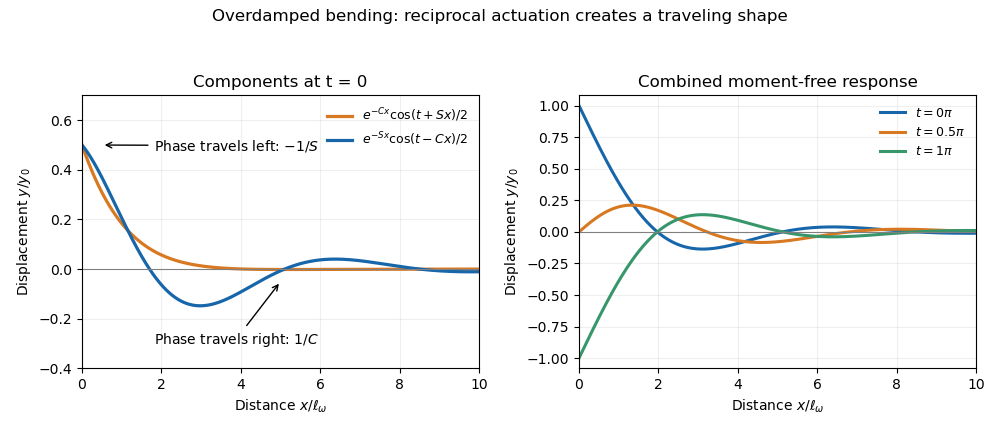
Codex 0 Created 2026-10-03 Updated 2026-10-14For the long filament, take the time-periodic solution of the dimensionless bending equation, after transients have decayed. Write . Then , so the spatial exponents satisfy . Define and . The two roots with negative real part are and ; the other roots violate decay at infinity.
Hence . The driven displacement gives , while the zero bending moment gives . Since , . The oscillatory bending of a moment-free semi-infinite filament isHolding each wave phase constant gives its dimensionless phase velocity:The first travels toward the actuator and attenuates over length ; the second travels away and attenuates over the longer length . These are spatially damped phase patterns in an overdamped bending equation, not two undamped inertial beam waves. Their combination satisfies both displacement and zero-moment conditions at the driven end.
Past exam of the mathematics course of the University of Cambridge 2019 iii Paper 334 2 c Solution by Codex 0 Created 2026-10-03 Updated 2026-10-05
Codex 0 Created 2026-10-03 Updated 2026-10-05A periodic displacement with angular frequency has . Balancing this viscous forcing with bending over length gives . Thus the elastohydrodynamic penetration length and sperm number areSince , the fourth root has dimensions length, as required.
With , , and , the bending equation becomesThe defining balance cancels both coefficients, giving . A large sperm number means that the periodically forced response decays before reaching the distant end.
Past exam of the mathematics course of the University of Cambridge 2019 iii Paper 334 2 b Solution by Codex 0 Created 2026-10-03 Updated 2026-10-05
Codex 0 Created 2026-10-03 Updated 2026-10-05In the small-slope Monge representation, , , and the leading transverse velocity is . With no imposed axial prestress, the induced filament tension is second order in transverse amplitude, so its transverse contribution is higher order. The transverse component of force balance reduces to the small-slope elastohydrodynamic filament equationAn externally imposed zeroth-order tension would instead add .
For the transverse motion, the off-diagonal part of the resistive-force theory tensor gives axial propulsive force density to second order. Its integral isSubstitute the bending equation and integrate by parts:The boundary expression for transverse filament thrust is thereforeOnly endpoint slope, bending moment, and shear enter this expression. Exact inextensibility also generates second-order longitudinal material motion; if that motion is retained in instantaneous total axial drag, it adds . For a periodic deformation with fixed axial base position, that additional term has zero cycle average. Thus the displayed formula is the transverse propulsive contribution and also gives the cycle-averaged propulsive force.
Past exam of the mathematics course of the University of Cambridge 2019 iii Paper 334 2 a Solution by Codex 0 Created 2026-10-03 Updated 2026-10-05
Codex 0 Created 2026-10-03 Updated 2026-10-05The first term is the local viscous force per unit length from resistive-force theory. With unit tangent vector , the drag tensor gives , where is velocity relative to the fluid.
The second term is the bending force of an inextensible filament. Varying its energy gives bulk force density . The final term, , is the force density from filament tension; is the Lagrange multiplier enforcing . At low Reynolds number, these forces balance without a filament acceleration term.
With mass, length, and time dimensions , the coefficients haveThus the drag coefficients have the dimensions of dynamic viscosity, the filament bending modulus has dimensions force times length squared, and tension has dimensions force.
Past exam of the mathematics course of the University of Cambridge 2019 iii Paper 334 1 g Solution by Codex 0 Created 2026-10-03 Updated 2026-10-14
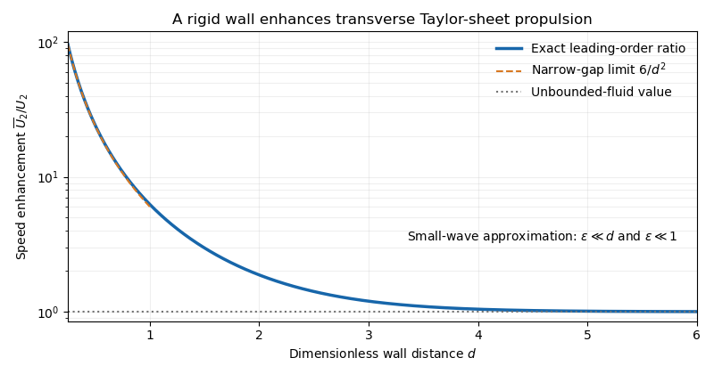
Codex 0 Created 2026-10-03 Updated 2026-10-14Since , the speed enhancement isThe strict inequality follows from . It tends to one as the wall recedes, while gives in a narrow gap. The wall enhances the mean pumping generated by transverse boundary motion. This small-amplitude limit requires ; letting the wall collide with a wave crest falls outside the expansion.
Wall enhancement of transverse-sheet swimming
. The leading swimming-speed ratio is greater than one for every finite gap and approaches one for a distant wall. The narrow-gap divergence is used only while the wave amplitude remains much smaller than the gap. Details. Past exam of the mathematics course of the University of Cambridge 2019 iii Paper 334 1 f Solution by Codex 0 Created 2026-10-03 Updated 2026-10-05
Codex 0 Created 2026-10-03 Updated 2026-10-05At the sheet, the second-order conditions are and . At the wall, and . The general solution has a polynomial mean mode and a second harmonic with exponentials , as in the unbounded calculation.
Let . The averaged Stokes equation, with periodic pressure and no imposed mean pressure gradient, gives . The total horizontal hydrodynamic force on the sheet is opposite to the mean shear force on the flat wall. Since the swimmer is force-free, , making the mean velocity constant. Matching its values at the sheet and wall therefore givesThe previous part gives , henceThis determines the speed without solving the second-harmonic flow. The force constraint matters: prescribing a translating sheet without imposing zero net force would allow a mean shear and would not determine a unique swimming speed.
Past exam of the mathematics course of the University of Cambridge 2019 iii Paper 334 1 e Solution by Codex 0 Created 2026-10-03 Updated 2026-10-05
Codex 0 Created 2026-10-03 Updated 2026-10-05The wall removes the far-field decay condition and instead imposes , . The force-free condition eliminates any first-order mean shear; since mean sheet tangential velocity is zero, . Thus , whereStart with the hyperbolic function form . The lower conditions give , . Defining , the wall conditions giveConsequently the first-order flow for Taylor-sheet swimming next to a rigid wall isFor , ensures a nonzero denominator; as , this reduces to the unbounded first-order field on every fixed height interval.
Past exam of the mathematics course of the University of Cambridge 2019 iii Paper 334 1 d Solution by Codex 0 Created 2026-10-03 Updated 2026-10-05
Codex 0 Created 2026-10-03 Updated 2026-10-05The wall is stationary in the laboratory and moves with velocity in the sheet frame. Its no-slip boundary condition is thereforeThe first equation prescribes wall tangential velocity; the second imposes zero normal velocity. The streamfunction may have a constant mean value on the wall, set by the fluid transport, and that constant need not equal its value at the sheet.
Past exam of the mathematics course of the University of Cambridge 2019 iii Paper 334 1 c Solution by Codex 0 Created 2026-10-03 Updated 2026-10-05
Codex 0 Created 2026-10-03 Updated 2026-10-05At second order the Taylor-expanded no-slip boundary condition iswith , , and at infinity. Set the irrelevant boundary constant to zero. The general relevant solution contains a zero Fourier mode and a second harmonic:Bounded velocity eliminates and growing harmonics. Averaging the tangential boundary condition gives . This is the mean boundary velocity determines Taylor-sheet swimming speed principle: the remaining mean velocity is uniform and equals the far-field velocity. ThereforeThe absence of odd powers follows because changing the amplitude sign is just a half-wavelength translation. Although unnecessary for the speed, the oscillatory solution can also be written explicitly as .
Past exam of the mathematics course of the University of Cambridge 2019 iii Paper 334 1 b Solution by Codex 0 Created 2026-10-03 Updated 2026-10-05
Codex 0 Created 2026-10-03 Updated 2026-10-05Expand and . A Taylor expansion of the sheet boundary conditions about givesThe first-order Fourier mode is , with , , and . Decay excludes the growing exponentials, leaving . The two boundary values give :There is no first-order mean boundary motion. Boundedness excludes mean shear, so .
Past exam of the mathematics course of the University of Cambridge 2019 iii Paper 334 1 a Solution by Codex 0 Created 2026-10-03 Updated 2026-10-05
Codex 0 Created 2026-10-03 Updated 2026-10-05Use the Cartesian streamfunction convention , . Taking the curl of the incompressible Stokes equation eliminates pressure and gives the biharmonic stream function for planar Stokes flow equationThe material points have no horizontal velocity in the swimming frame and have vertical velocity . The no-slip boundary condition is thereforeAt infinity the laboratory fluid is at rest, so in this translating frame it moves with :Velocity and its perturbations are periodic in , with period , and the pressure has no imposed mean gradient. The Taylor swimming sheet is force-free; the unbounded problem's bounded far-field velocity enforces the absence of mean shear. An additive constant in the streamfunction has no physical effect.
Pinned article: Introduction to the OurBigBook Project
Welcome to the OurBigBook Project! Our goal is to create the perfect publishing platform for STEM subjects, and get university-level students to write the best free STEM tutorials ever.
Everyone is welcome to create an account and play with the site: ourbigbook.com/go/register. We belive that students themselves can write amazing tutorials, but teachers are welcome too. You can write about anything you want, it doesn't have to be STEM or even educational. Silly test content is very welcome and you won't be penalized in any way. Just keep it legal!
Intro to OurBigBook
. Source. We have two killer features:
- topics: topics group articles by different users with the same title, e.g. here is the topic for the "Fundamental Theorem of Calculus" ourbigbook.com/go/topic/fundamental-theorem-of-calculusArticles of different users are sorted by upvote within each article page. This feature is a bit like:
- a Wikipedia where each user can have their own version of each article
- a Q&A website like Stack Overflow, where multiple people can give their views on a given topic, and the best ones are sorted by upvote. Except you don't need to wait for someone to ask first, and any topic goes, no matter how narrow or broad
This feature makes it possible for readers to find better explanations of any topic created by other writers. And it allows writers to create an explanation in a place that readers might actually find it.
Figure 1. Screenshot of the "Derivative" topic page. View it live at: ourbigbook.com/go/topic/derivativeVideo 2. OurBigBook Web topics demo. Source. - local editing: you can store all your personal knowledge base content locally in a plaintext markup format that can be edited locally and published either:This way you can be sure that even if OurBigBook.com were to go down one day (which we have no plans to do as it is quite cheap to host!), your content will still be perfectly readable as a static site.
- to OurBigBook.com to get awesome multi-user features like topics and likes
- as HTML files to a static website, which you can host yourself for free on many external providers like GitHub Pages, and remain in full control

Figure 2. You can publish local OurBigBook lightweight markup files to either OurBigBook.com or as a static website.
Figure 3. Visual Studio Code extension installation.
Figure 5. . You can also edit articles on the Web editor without installing anything locally. Video 3. Edit locally and publish demo. Source. This shows editing OurBigBook Markup and publishing it using the Visual Studio Code extension. 
- Infinitely deep tables of contents:




All our software is open source and hosted at: github.com/ourbigbook/ourbigbook
Further documentation can be found at: docs.ourbigbook.com
Feel free to reach our to us for any help or suggestions: docs.ourbigbook.com/#contact