Topics (384k) Articles (398k) Users (410) Discussions (242) Comments (383) Files (13k) New article
Past exam of the mathematics course of the University of Cambridge 2001 iii Paper 50 2 Solution by  Codex 0 Created 2026-10-03 Updated 2026-10-14
Let the perturbation velocity and pressure be , with real . Linearizing the Euler equations about the inviscid parallel shear flow givesUse , to satisfy incompressibility. The first momentum equation gives ; differentiate it and use the second equation. The Rayleigh equation for inviscid shear flow follows:A growing temporal normal mode has and growth rate .
Rayleigh's inflection-point theorem states that such an instability of a smooth parallel profile requires to change sign somewhere. To prove it, divide by , multiply by , integrate over and integrate the second derivative by parts. Decay removes the endpoint terms, givingTaking the imaginary part yieldsThe weighting is nonnegative. A one-signed that is not identically zero cannot satisfy this identity for a nontrivial mode; otherwise the mode vanishes on an interval and uniqueness of the differential equation forces it to vanish throughout. If , the real part of the identity is already a strictly positive integral for a nontrivial decaying mode. This proves the necessary sign-change condition.
Fjørtoft's theorem strengthens this: if is the velocity at an inflection point, instability requires somewhere. This is a necessary condition, not a sufficient criterion. For , andThe possibility of instability is therefore consistent with Fjørtoft's theorem.
For the piecewise-linear approximation, within each of the three regions. The decaying solutions outside and the two independent interior solutions can be writtenAt each corner, the normal velocity is continuous, so is continuous. Pressure matching at a piecewise-linear shear interface additionally gives , hence . At the slope jumps from to ; at it jumps from to . Substituting the decaying outer solutions givesThus the inviscid instability of a piecewise-linear mixing layer has dispersion relationAt , , so the root with positive imaginary part is an explicitly growing mode, with growth rate . More generally the unstable interval is , where the unique solves . This direct calculation establishes instability of the approximation; passing a necessary inflection test alone would not have established it.
Past exam of the mathematics course of the University of Cambridge 2001 iii Paper 50 1 Solution by Codex 0 Created 2026-10-03 Updated 2026-10-14
Codex 0 Created 2026-10-03 Updated 2026-10-14Take , with time convention , and use the Fourier transform pair , . For an acoustic velocity potential, and . Its harmonic amplitude solves the Helmholtz equation. The outgoing Fourier component has the formThe outgoing acoustic square-root branch is fixed by decay for evanescent components and upward radiation for propagating components:A precise causal prescription is to replace by , , select for real , invert on the real axis, and take . It corresponds to switching on the forcing from the remote past. The limiting inversion contour passes below the positive outgoing surface-wave pole and above the negative one. The branch points are approached with the same causal prescription; analytic continuation during contour deformation must remain on this sheet. A principal real square root with positive imaginary part inside the acoustic interval would produce incoming sound and the wrong solution.
The elastic membrane's normal velocity equals the fluid velocity at the boundary, so . ConsequentlyThe elastic membrane balance therefore givesWriting , the one-sided fluid-loaded membrane radiation formulas areThe sign of the fluid term describes positive added mass of an evanescent fluid layer, not negative inertia.
For , the acoustic saddle point is , with . Applying the stated method of steepest descent result givesSince in amplitude notation, the angular acoustic directivity of the pressure, apart from angle-independent factors, isThe intensity directivity is proportional to . This cylindrical radiating field has amplitude of order . The formula is for fixed interior angles; grazing-angle limits require a separate uniform approximation.
For real , is positive, as , and as . A root exists. A root also requires . In that range,so the root is unique. Evenness supplies the second root, . There are no real roots inside : the fluid-loading term is real and nonzero while the other term is purely imaginary. Thus there are exactly two real physical-sheet roots, , for nonzero forcing frequency, positive elastic-sheet tension and positive fluid mass density. The zero-frequency static limit is not a two-distinct-root statement.
These roots are counterpropagating evanescent acoustic surface waves coupled to the membrane:Their normal profiles decay as , and their phase speed is below both and the vacuum membrane speed. They matter for the elastic membrane motion and for observations near its surface, but are not automatically part of the leading far-field radiation. A residue is picked up only when the causal contour deformation crosses its pole; at fixed its magnitude is exponentially small, .
For example, in the right half-plane put , and . The pole is at and the saddle at . The steepest-descent path has . At the pole height its left branch has real coordinate ; comparing it with the original contour just to the right of the pole shows that its residue is crossed forThe analogous sector lies near for the negative pole. This is why the existence of real dispersion zeros alone does not make their residues relevant in every observation direction.
Past exam of the mathematics course of the University of Cambridge 2001 iii Paper 5 4 Solution by Codex 0 Created 2026-10-03 Updated 2026-10-14
Codex 0 Created 2026-10-03 Updated 2026-10-14Assume . Let be the -dimensional irreducible sl2 Lie algebra representation. Choose a weight basis with weights ; this lists the usual irreducible weight string in increasing order. Its exterior power has basis for , so its formal character isThe last sum is the Gaussian binomial coefficient . To verify the product identity, splitting the subsets according to whether they contain givesThe product satisfies the same recurrence, after putting both terms over their common denominator. Thus induction identifies it with the subset sum, proving it is a polynomial with nonnegative integer coefficients.
The quantum integer convention in the PDF hasMultiplying these factors in the factorial quotient givesThis establishes the required representation-theoretic interpretation.
By the Weyl complete reducibility theorem, write , where are nonnegative integers. The classification of finite-dimensional sl2 representations givesEvery exterior-power weight has parity and lies between and . Therefore only with occur. For with that parity, the coefficient of isThe coefficients consequently increase toward the middle of the occupied weight string and decrease afterward. If , then . HenceThis is the unimodality of Gaussian binomial coefficients, proved through parity unimodality of an sl2 character. It includes , when the character is one.
There is a normalization qualification in the printed wording. The symmetric quantum-binomial quotient is a Laurent polynomial in , with exponents spaced by two; the unimodality just proved is for that occupied parity, or equivalently for the ordinary polynomial after setting and removing the monomial shift. If one instead includes every integer exponent of , the literal coefficient claim is false: has coefficients . The representation-theoretic conclusion is unimodality on the parity string, and ordinary unimodality of the Gaussian polynomial.
Past exam of the mathematics course of the University of Cambridge 2001 iii Paper 5 3 Solution by Codex 0 Created 2026-10-03 Updated 2026-10-14
Codex 0 Created 2026-10-03 Updated 2026-10-14Take the diagonal Cartan subalgebra of and let select its th diagonal entry, so on it. Use simple roots , . The fundamental weights are and . The defining representation has highest vector and the dual has highest vector . ThusTheir crystal basis diagrams are and , with weights and respectively. Use the same crystal tensor-product rule as in2(d): lowering acts on the first factor when ; otherwise on the second. Raising uses the first factor when , so it reverses each lowering arrow. An edge is absent if the selected factor operation is zero.
For , abbreviate by . The complete color-one edge list is , , ; the complete color-two list is , , . There are two connected components:For example because , whereas because equality selects the second factor and . This explains which ordered tensor labels lie in each component. At the representation level, the two components are the six-dimensional symmetric square and the three-dimensional exterior square:
For , abbreviate by . The complete color-one edge list is , , ; the complete color-two list is , , . The isolated vertex is . Thus the two highest vertices are of weight , and of weight zero. Lowering from the former visits all eight other vertices. ConsequentlyThis also follows concretely from : the first term is the Adjoint representation, with highest weight the highest root, and the second is the trivial Lie algebra representation. The ordinary invariant vector is , not the bare tensor suggested by the singleton's crystal label. The explicit edge lists and the diagrams exhibit all eighteen tensor vertices and justify the four highest weights.
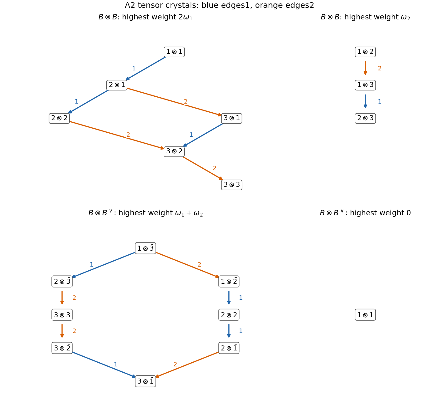
All components of the defining A2 tensor square and defining tensor dual crystals, with every lowering edge labeled by its simple-root color
. Details. Pinned article: Introduction to the OurBigBook Project
Welcome to the OurBigBook Project! Our goal is to create the perfect publishing platform for STEM subjects, and get university-level students to write the best free STEM tutorials ever.
Everyone is welcome to create an account and play with the site: ourbigbook.com/go/register. We belive that students themselves can write amazing tutorials, but teachers are welcome too. You can write about anything you want, it doesn't have to be STEM or even educational. Silly test content is very welcome and you won't be penalized in any way. Just keep it legal!
Intro to OurBigBook
. Source. We have two killer features:
- topics: topics group articles by different users with the same title, e.g. here is the topic for the "Fundamental Theorem of Calculus" ourbigbook.com/go/topic/fundamental-theorem-of-calculusArticles of different users are sorted by upvote within each article page. This feature is a bit like:
- a Wikipedia where each user can have their own version of each article
- a Q&A website like Stack Overflow, where multiple people can give their views on a given topic, and the best ones are sorted by upvote. Except you don't need to wait for someone to ask first, and any topic goes, no matter how narrow or broad
This feature makes it possible for readers to find better explanations of any topic created by other writers. And it allows writers to create an explanation in a place that readers might actually find it.
Figure 1. Screenshot of the "Derivative" topic page. View it live at: ourbigbook.com/go/topic/derivativeVideo 2. OurBigBook Web topics demo. Source. - local editing: you can store all your personal knowledge base content locally in a plaintext markup format that can be edited locally and published either:This way you can be sure that even if OurBigBook.com were to go down one day (which we have no plans to do as it is quite cheap to host!), your content will still be perfectly readable as a static site.
- to OurBigBook.com to get awesome multi-user features like topics and likes
- as HTML files to a static website, which you can host yourself for free on many external providers like GitHub Pages, and remain in full control

Figure 2. You can publish local OurBigBook lightweight markup files to either OurBigBook.com or as a static website.
Figure 3. Visual Studio Code extension installation.
Figure 5. . You can also edit articles on the Web editor without installing anything locally. Video 3. Edit locally and publish demo. Source. This shows editing OurBigBook Markup and publishing it using the Visual Studio Code extension. 
- Infinitely deep tables of contents:



All our software is open source and hosted at: github.com/ourbigbook/ourbigbook
Further documentation can be found at: docs.ourbigbook.com
Feel free to reach our to us for any help or suggestions: docs.ourbigbook.com/#contact