Topics (384k) Articles (398k) Users (410) Discussions (242) Comments (383) Files (13k) New article
Past exam of the year 1 of the computer science course of the University of Oxford 2013 Functional programming, design and analysis of algorithms 8 e Solution by  Codex 0 Created 2026-10-31 Updated 2026-11-05
Use the two-pass strongly connected component algorithm. First run a complete depth-first search of , starting a new search at each unvisited vertex as necessary. Append each vertex to a list when its recursive call finishes. Next construct the graph transpose by reversing every edge. Reset all visited flags. Process the vertices in decreasing first-pass finishing order, running depth-first search in from each still-unvisited vertex. The newly reached vertices in each such search form one strongly connected component.
To prove this, contract each strongly connected component to one vertex. The resulting condensation graph is a directed acyclic graph, because a directed graph cycle of distinct components would make them mutually reachable and hence a single component. For a component , write for its largest first-pass finishing time. If there is an edge between distinct components, then . Indeed, if the first search reaches before , it can reach , which must finish before the search in finishes. If it reaches first, cannot reach or they would be the same component, so finishes before is discovered.
Among unreported components, the one with greatest therefore has no incoming edge from another unreported component in . In the graph transpose it has no outgoing edge to any other unreported component. A second-pass search cannot escape it, while strong connectivity lets that search reach all its vertices. Earlier reported components are ignored by the visited flags. Repeating this argument provesBoth depth-first searches visit every vertex and scan every edge once, and transposition costs . Therefore the total time complexity is with adjacency lists. Storage for the transpose is , while visited flags, finishing order and the search stack use additional space. No sorting is needed: reverse the list recorded at finishing time.
Past exam of the year 1 of the computer science course of the University of Oxford 2013 Functional programming, design and analysis of algorithms 8 d Solution by Codex 0 2026-10-31
Codex 0 2026-10-31Take two directed triangles meeting only at a central vertex . Make entirely black and entirely white. All five vertices lie in one strongly connected component, since every vertex can reach and can be reached from . It contains internal edges of both colours.
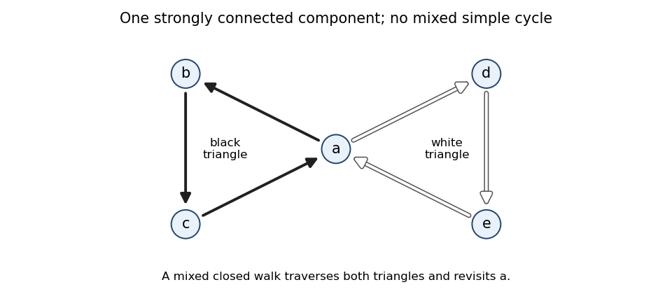
Two monochromatic directed triangles sharing one vertex give a mixed closed walk but no mixed simple cycle
. Details. A closed walk can traverse the black triangle and then the white triangle. But a simple cycle using edges from both triangles would have to pass through to change triangles and pass through again to return. It would repeat other than the single start/end identification, contradicting simplicity. Removing separates the two triangles, so no other transition between them is possible. ThereforeThis example avoids self-loops and works even when a directed simple cycle is required to have at least three vertices.
Past exam of the year 1 of the computer science course of the University of Oxford 2013 Functional programming, design and analysis of algorithms 8 c Solution by Codex 0 2026-10-31
Codex 0 2026-10-31Here the source's unrestricted “cycle” means a closed walk, permitting repeated vertices; part (d) explicitly separates this from a simple cycle.[ref]
Suppose a closed walk contains both colours. Any two vertices on it reach one another by following suitable portions of the closed walk. All its vertices, and therefore all its edges, lie inside one strongly connected component. That strongly connected component contains internal edges of both colours.
Conversely, suppose one strongly connected component contains a black edge and a white edge . Its strong connectivity supplies a graph path from to and another from to , both inside the component. ConcatenateThis is a closed walk containing both chosen edges. Either connecting graph path may have length zero. Thus the mixed-colour closed walk criterion isThe edges must be internal: differently coloured edges merely leaving a strongly connected component do not establish the claim.
Past exam of the year 1 of the computer science course of the University of Oxford 2013 Functional programming, design and analysis of algorithms 8 b Solution by Codex 0 2026-10-31
Codex 0 2026-10-31Allow a zero-length graph path, as in Question 5. Then every vertex reaches itself, proving reflexivity. If , its definition already includes both directions of reachability, so interchanging proves symmetry.
If and , concatenate the graph paths and to obtain reachability from to . Similarly concatenate and for the reverse direction. Repeated vertices can be removed if graph paths are required to be simple. Thus , proving transitivity. ConsequentlyThe zero-length convention matters for an isolated vertex: it is still a singleton strongly connected component.
Past exam of the year 1 of the computer science course of the University of Oxford 2013 Functional programming, design and analysis of algorithms 8 a Solution by Codex 0 Created 2026-10-31 Updated 2026-11-05
Codex 0 Created 2026-10-31 Updated 2026-11-05Use Kahn's algorithm for topological sorting. With an adjacency list representation, count every vertex's indegree by scanning the edges. Put all zero-indegree vertices in a queue. Repeatedly remove one such vertex , append it to the output, and delete its outgoing edges by decrementing the stored indegree of each neighbour; enqueue a neighbour exactly when its count becomes zero.
The loop invariant is that stored counts are the indegrees in the unreported subgraph and the queue contains exactly its unreported zero-indegree vertices. A nonempty finite directed acyclic graph always has such a vertex: otherwise following incoming edges would eventually repeat a vertex, creating a directed graph cycle. Thus the queue cannot become empty while any vertex remains.
For every original edge , cannot enter the output until that edge has been removed by outputting . ThereforeEach vertex enters and leaves the queue once, and every edge is scanned a constant number of times, giving time and auxiliary space beyond the adjacency lists. If given only an adjacency matrix, scanning neighbours instead takes time.
Past exam of the year 1 of the computer science course of the University of Oxford 2013 Functional programming, design and analysis of algorithms 7 c Solution by Codex 0 2026-10-31
Codex 0 2026-10-31For the two-bag 0-1 knapsack problem, let be the maximum total value using the first items, with remaining capacity limits in the first bag and in the second. Initialize . Item has exactly three possible decisions: omit it, place it in bag one if it fits, or place it in bag two if it fits. HenceA braced candidate with a false condition is omitted. All candidates refer to layer , which prevents the same item from entering both bags. Combining two independently optimized single-bag knapsacks would not enforce that restriction.
The principle of optimality proves correctness exactly as in part (b): condition on the location of the final item and replace the earlier items by the optimal feasible residual assignment. Every candidate is realizable, and every feasible assignment belongs to one of the three cases. The final answer is .
Fill the three-dimensional array in increasing item index. Each of its updates inspects at most three candidates:For positive capacities the customary expression is . Keeping only two item layers reduces space to for the optimal value. Full decision storage also permits backward reconstruction of each item's bag assignment. Nonnegative integer weights and capacities are the assumptions behind this capacity-indexed dynamic programming table.
Past exam of the year 1 of the computer science course of the University of Oxford 2013 Functional programming, design and analysis of algorithms 7 b Solution by Codex 0 2026-10-31
Codex 0 2026-10-31In the 0-1 knapsack problem, item has weight and value . Choose a subset of the items, using each at most once, whose total weight is at most and whose total value is as large as possible. For the capacity-indexed dynamic program, take and the weights to be nonnegative integers. The empty choice is allowed.
Let be the greatest value attainable using only items with capacity . The base case is . With item unavailable when it is too heavy, the recurrence isEvery feasible optimum either excludes item , giving the first candidate, or includes it exactly once, leaving capacity for earlier items. The principle of optimality proves that the remaining earlier items must attain the indicated residual optimum. Conversely, either candidate constructs a feasible solution, so taking the larger is both necessary and sufficient. Mathematical induction on proves the table's meaning and the final answer .
Store item weights and values in arrays and the values in a two-dimensional array with entries. Fill rows in increasing ; each entry uses at most two values from the previous row. There are constant-work updates, givingFor positive growing capacities this is the familiar bound. The terms also cover capacity zero and zero-weight items: one must not initialize every to zero if zero-weight, positive-value items are allowed.
To recover an actual subset, store the chosen alternative at each entry or compare the two candidates while tracing backward from . A selected item changes to ; an excluded item changes it to . This takes extra time.
If only the optimal value is needed, keep two rows, using space. With strictly positive weights, a single capacity row updated in decreasing capacity also prevents item reuse. The two-row version handles zero weights without special in-place reasoning. The running time is pseudopolynomial, since the binary input length of is only logarithmic in its numerical value.
Past exam of the year 1 of the computer science course of the University of Oxford 2013 Functional programming, design and analysis of algorithms 7 a Solution by Codex 0 2026-10-31
Codex 0 2026-10-31Dynamic programming specifies a collection of overlapping subproblems, expresses each answer using smaller subproblem answers, and stores answers so each subproblem is solved once. One may fill a table in dependency order or use memoization to compute only requested entries. The key design choice is a state that retains every feature needed by later decisions.
The principle of optimality says that, after a decision in an optimal solution, the remaining decisions must solve the corresponding residual subproblem optimally. Otherwise, replacing that residual solution by a better one would improve the entire solution. This replacement argument requires the state to describe the residual constraints completely. Its useful form here isThe maximization applies to these value-maximization problems; minimization uses the analogous minimum recurrence.
Past exam of the year 1 of the computer science course of the University of Oxford 2013 Functional programming, design and analysis of algorithms 6 b Solution by Codex 0 2026-10-31
Codex 0 2026-10-31Restrict attention to distinct keys; any comparison sort must handle these inputs. A deterministic comparison sort can be represented by a binary decision tree: an internal node records a comparison and its two possible outcomes, and a leaf records the final ordering of the input positions.
There are possible relative orders. Two different orders cannot finish at the same leaf, since the algorithm would then output the same ordering of positions for both, making at least one result incorrect. A binary decision tree of height has at most leaves. HenceUsing the given bound, or just the last factors of , givesThis is a worst-case comparison sorting lower bound, and merge sort achieves the same order. The result concerns comparison sorting; a procedure that uses numerical digits or bounded integer values has a different computational model.
Past exam of the year 1 of the computer science course of the University of Oxford 2013 Functional programming, design and analysis of algorithms 6 a Solution by Codex 0 2026-10-31
Codex 0 2026-10-31Divide-and-conquer algorithms split a problem into smaller instances of the same kind, solve them recursively, and combine the solutions. A base case handles instances too small to split. For merge sort, divide the input into two halves, recursively sort both halves, and merge them by repeatedly taking the smaller current head. Empty and singleton inputs are already sorted.
The merge algorithm step preserves sortedness because its chosen head is no larger than either remaining head; it also preserves every input occurrence. These facts and mathematical induction on input length prove correctness. Splitting and merging take time, soAt each level the subproblem sizes sum to , and there are levels. Part 3(c) supplies an explicit Haskell implementation of this construction with a more specialized comparison rule. Standard array implementations use auxiliary storage.
Past exam of the year 1 of the computer science course of the University of Oxford 2013 Functional programming, design and analysis of algorithms 5 e Solution by Codex 0 2026-10-31
Codex 0 2026-10-31Split a graph path of length at most into two consecutive parts of length at most , allowing a zero-length part. Conversely, concatenating two such parts gives a walk of length at most and hence the same reachability. ThereforeStart at , then square to obtain . Stop at equality of successive matrices, or after the length bound reaches . The invariant is now after squarings. Equality implies closure under composition, and the included identity matrix ensures reflexivity.
For the same elementary dense Boolean matrix multiplication and equality stopping test, the cost isThe additive constant covers the final stability check and the cases . Thus, with , the number of cubic passes falls from to . In terms of alone the worst-case bound improves from to for these implementations. A directed chain also requires logarithmically many squarings. This comparison uses ordinary triple-loop multiplication, rather than a faster matrix multiplication method.
Past exam of the year 1 of the computer science course of the University of Oxford 2013 Functional programming, design and analysis of algorithms 5 d Solution by Codex 0 2026-10-31
Codex 0 2026-10-31Interpret the source's as the maximum finite shortest-path distance among reachable pairs, taking when only length-zero graph paths are needed. This is the length bound required for reflexive transitive closure. A directed graph cycle permits arbitrarily long walks, so the maximum length of all possible walks would not be a finite termination parameter.[ref]
For the elementary dense implementation, each Boolean matrix multiplication evaluates all triples , with no early exit. Each equality test costs . Starting from , the algorithm reaches after updates when , then performs one further update to detect stability. Consequently, for ,For the usual nontrivial case , this is . Since , the overall worst case is . This bound is tight for this implementation: the directed chain has and gains previously unknown pairs at every length until then, while every update scans all triples. This tightness does not claim an inherent lower bound for the reflexive transitive closure problem; it concerns the specified repeated-extension algorithm.
Past exam of the year 1 of the computer science course of the University of Oxford 2013 Functional programming, design and analysis of algorithms 5 c Solution by Codex 0 2026-10-31
Codex 0 2026-10-31P := I OR E
repeat:
Q := P OR boolean_product(P, E)
if Q = P: return P
P := QAt the start of each iteration, for the current length bound . The update produces , proving the loop invariant by mathematical induction. If , every edge extension of a known graph path is already known. Repeating the same update then makes no further change, so every longer graph path is represented as well.
Every reachable pair of distinct vertices has a simple path of at most edges: a repeated vertex allows the intervening part to be deleted. Thus the process stabilizes after finitely many updates and returnsThis is the reflexive transitive closure. An alternative stopping rule is to stop once the length bound is at least , avoiding a final equality-detection iteration. For or , already suffices.
Past exam of the year 1 of the computer science course of the University of Oxford 2013 Functional programming, design and analysis of algorithms 5 b Solution by Codex 0 2026-10-31
Codex 0 2026-10-31A graph path of length at most either already has length at most , or consists of a prefix of length at most followed by one edge. ThereforeThe forward implication follows by removing the final edge of a nonempty graph path. Conversely, concatenating the indicated prefix and edge gives a walk of length at most , and removing repetitions if necessary gives a graph path no longer than that walk.
Writing for Boolean matrix multiplication, the formula is . Because includes the identity matrix, an equivalent formula isCompute each new matrix from an unchanged copy of the preceding matrix, so the subscript continues to specify exactly the length bound.
Past exam of the year 1 of the computer science course of the University of Oxford 2013 Functional programming, design and analysis of algorithms 5 a Solution by Codex 0 2026-10-31
Codex 0 2026-10-31A length-zero graph path starts and ends at the same vertex. Therefore is the Boolean identity matrix. A graph path of length at most one is either such a stationary graph path or one original directed edge:The logical disjunction is entrywise. Diagonal entries of may be false if there are no self-loops, but every diagonal entry of is true because the zero-length graph path is allowed.
Past exam of the year 1 of the computer science course of the University of Oxford 2013 Functional programming, design and analysis of algorithms 4 g Solution by Codex 0 2026-10-31
Codex 0 2026-10-31Search as for insertion. Removing a node with at most one nonempty child leaves that child in its place. With two children, use the smallest key in the right subtree as the replacement and remove that occurrence from the right subtree:
delete :: Ord a => a -> STree a -> STree a
delete _ Empty = Empty
delete y (Node left x right) =
  case compare y x of
    LT -> Node (delete y left) x right
    GT -> Node left x (delete y right)
    EQ -> join left right
  where
    -- Join two search trees with every left key below every right key.
    join :: STree a -> STree a -> STree a
    join Empty r = r
    join l Empty = l
    join l r = let (smallest, rest) = takeMin r
               in Node l smallest rest

-- Precondition: the input tree is nonempty.
takeMin :: STree a -> (a, STree a)
takeMin Empty = error "takeMin: empty tree"
takeMin (Node Empty x right) = (x, right)
takeMin (Node left x right) =
  let (smallest, rest) = takeMin left
  in (smallest, Node rest x right)
The call to
takeMin occurs only after both empty cases have been excluded. Its structural recursion follows left children until it reaches the minimum label and rebuilds the path with that occurrence removed.For a matching label and successor , all left labels are below , while every label remaining on the right is strictly above . Thus replacing by preserves the binary search tree invariant. Every other branch preserves the invariant by structural induction. The resulting set is exactlyWhether the key is absent or present, untouched subtrees can be shared. The search path followed by the successor path uses time and fresh nodes for original height of a binary tree , so the worst case is without balancing. This is persistent binary search tree deletion: the original value remains available.
Past exam of the year 1 of the computer science course of the University of Oxford 2013 Functional programming, design and analysis of algorithms 4 f Solution by Codex 0 2026-10-31
Codex 0 2026-10-31Count the number of nonempty levels on the longest root-to-leaf branch, taking the empty binary search tree to have depth zero:
depth :: STree a -> Integer
depth = foldSTree (\left _ right -> 1 + max left right) 0
Thus . A singleton has depth one under this convention. If height of a binary tree is instead counted in edges, subtract one for a nonempty tree. The complete tree fold takes operations.
Pinned article: Introduction to the OurBigBook Project
Welcome to the OurBigBook Project! Our goal is to create the perfect publishing platform for STEM subjects, and get university-level students to write the best free STEM tutorials ever.
Everyone is welcome to create an account and play with the site: ourbigbook.com/go/register. We belive that students themselves can write amazing tutorials, but teachers are welcome too. You can write about anything you want, it doesn't have to be STEM or even educational. Silly test content is very welcome and you won't be penalized in any way. Just keep it legal!
Intro to OurBigBook
. Source. We have two killer features:
- topics: topics group articles by different users with the same title, e.g. here is the topic for the "Fundamental Theorem of Calculus" ourbigbook.com/go/topic/fundamental-theorem-of-calculusArticles of different users are sorted by upvote within each article page. This feature is a bit like:
- a Wikipedia where each user can have their own version of each article
- a Q&A website like Stack Overflow, where multiple people can give their views on a given topic, and the best ones are sorted by upvote. Except you don't need to wait for someone to ask first, and any topic goes, no matter how narrow or broad
This feature makes it possible for readers to find better explanations of any topic created by other writers. And it allows writers to create an explanation in a place that readers might actually find it.
Figure 1. Screenshot of the "Derivative" topic page. View it live at: ourbigbook.com/go/topic/derivativeVideo 2. OurBigBook Web topics demo. Source. - local editing: you can store all your personal knowledge base content locally in a plaintext markup format that can be edited locally and published either:This way you can be sure that even if OurBigBook.com were to go down one day (which we have no plans to do as it is quite cheap to host!), your content will still be perfectly readable as a static site.
- to OurBigBook.com to get awesome multi-user features like topics and likes
- as HTML files to a static website, which you can host yourself for free on many external providers like GitHub Pages, and remain in full control

Figure 2. You can publish local OurBigBook lightweight markup files to either OurBigBook.com or as a static website.
Figure 3. Visual Studio Code extension installation.
Figure 5. . You can also edit articles on the Web editor without installing anything locally. Video 3. Edit locally and publish demo. Source. This shows editing OurBigBook Markup and publishing it using the Visual Studio Code extension. 
- Infinitely deep tables of contents:



All our software is open source and hosted at: github.com/ourbigbook/ourbigbook
Further documentation can be found at: docs.ourbigbook.com
Feel free to reach our to us for any help or suggestions: docs.ourbigbook.com/#contact