
The Bayesian posterior is the conditional probability distribution of an unknown statistical parameter after observing data. Suppose a continuous prior distribution has prior density relative to Lebesgue measure , and is the sampling probability mass function or probability density function of the observed data in the statistical model. Bayes' theorem givesThe Bayesian model evidence is the normalization constant making the posterior density integrate to one. The strict positive, finite condition is essential: a zero or infinite normalizer does not define this posterior distribution, even if the unnormalized expression can be written down. Other reference measures give the corresponding density formula; discrete parameter values replace the integral by a sum. The posterior propriety article gives examples where normalization fails.
With fixed, is a likelihood function of . Its normalization as a sampling distribution is over possible data, not over parameter values. In particular, a likelihood function is not a probability density function for and need not integrate to one over . The prior density supplies the probability weighting, and the Bayesian model evidence normalizes their product. This distinction prevents a tempting mistake: reversing the conditioning merely by exchanging the words “data” and “parameter”.
For eight heads among ten conditionally independent Bernoulli trials, take the observed data to be the heads count . Its binomial distribution likelihood function and the prior density giveUsing the Euler beta function , the Bayesian model evidence and normalized posterior density areThus the posterior distribution is . If the data are instead one particular ordered sequence with eight heads and two tails, its likelihood function omits the factor 45 and its Bayesian model evidence becomes . The factor cancels in Bayes' theorem, leaving the same posterior distribution; these two data descriptions have different sampling probabilities but identical information about here.
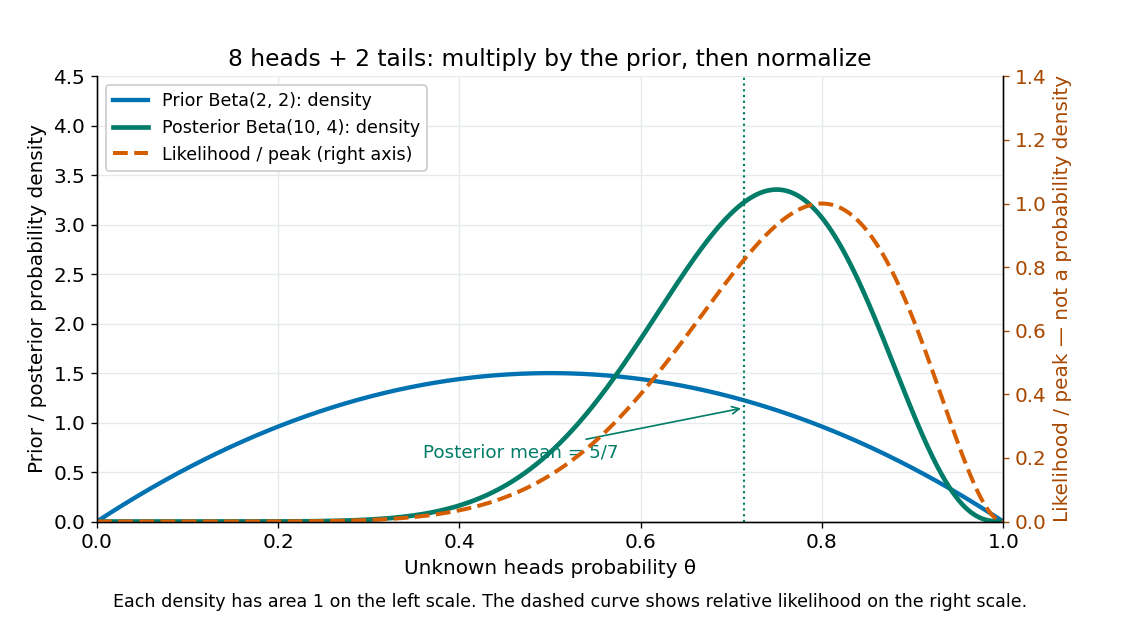
Beta(2,2) prior, peak-normalized Bernoulli likelihood, and Beta(10,4) posterior after eight heads and two tails
. Details. 
The prior density and posterior density use the left axis and each integrate to one. The dashed likelihood function uses the right axis and is divided by its maximum solely to compare its shape; it is not a parameter probability density function. The likelihood function peaks at , while the posterior mode is and the posterior mean is . Multiplying by the prior density shifts the preferred values toward one half while preserving a range of possibilities.
The resulting posterior variance is , compared with prior variance . In this example the update reduces uncertainty. The posterior predictive probability of heads on the next conditionally independent toss is , and the credible interval above reports a 95% range. These are summaries of the same posterior distribution, rather than competing estimates of one density peak.
New to topics? Read the docs here!