 Sinusoidal steady state

The sinusoidal steady state of a stable linear time-invariant system driven by a sinusoid is its persistent response at the driving frequency, after the relevant transient response has decayed. A phasor calculation finds that response; it does not generally satisfy the circuit's switch-on initial conditions. The late-time assumption is explicit in Berggren's treatment of sinusoidal circuit analysis.^[ref]

Using peak phasors, write the source as $v_s(t)=\mathrm{Re}({\hat{V}}_s{e}^{i\omega t})$. If $H(i\omega )$ is the relevant transfer function, its particular solution isThe complete response adds a homogeneous solution determined by the initial conditions. Approaching the displayed expression requires the modes affecting the measured output to decay; an unchanged amplitude and a fixed phase shift then characterize its frequency response.

For an original turn-on example, drive a series RC circuit with $v_s(t)=V_0\cos \omega t$ for $t\ge 0$, measure the capacitor's electric potential difference, and take $v_C(0)=0$. With time constant $\tau =RC>0$, Kirchhoff's voltage law gives the first-order linear differential equationPut $x=\omega \tau$. Substitution verifies the sinusoidal particular solution $V_0(\cos \omega t+x\sin \omega t)/(1+x^2)$. Adding $A{e}^{-t/\tau }$ and imposing the initial condition fixes $A=-V_0/(1+x^2)$, givingIts sinusoidal part has amplitude $V_0/\sqrt{1+x^2}$ and lags by $\arctan x$. The exponential settling bound for RC sinusoidal turn-on, relative to that amplitude, isWith chosen $R=1\mathrm{k\Omega }$, $C=1\mu \mathrm{F}$, $V_0=1\mathrm{V}$ and $\omega =1000rad/s$, we have $\tau =1\mathrm{ms}$ and $x=1$. At turn-on the phasor approximation predicts 0.5 volt while the capacitor is initially at zero. After 5 milliseconds, their difference is about 3.37 millivolts, or 0.476 percent of the sinusoidal amplitude. A 1 percent settling time threshold for this specific switch-on is about $4.259\tau$.

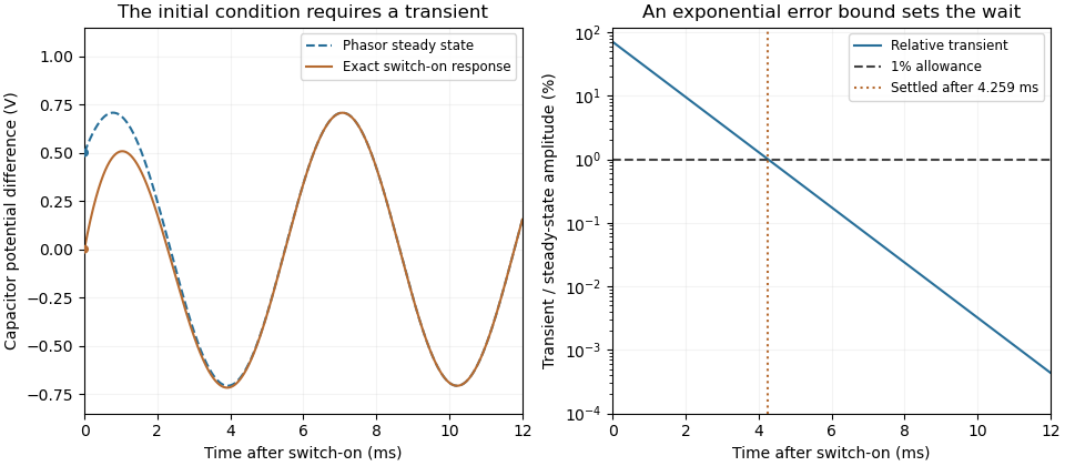
A useful measurement compares a long, low-frequency square-wave response with sinusoidal responses at several frequencies. An oscilloscope can identify the exponential decay and then measure amplitude ratios and phase shifts. MIT's laboratory uses that sequence to connect the time constant to the sinusoidal response; probe loading belongs in the measured circuit model.^[ref]

Undamped resonant forcing has no bounded sinusoidal steady state. For an ideal series LC circuit, let $q$ be electric charge and ${\omega }_0=1/\sqrt{LC}$. At resonance, the equationhas the particular solution $q_p(t)=V_{0}t\sin ({\omega }_{0}t)/(2L{\omega }_0)$. Its growing envelope prevents a bounded attracting sinusoidal response. This ideal counterexample explains why decay of the relevant homogeneous solutions is part of the physical steady-state assumption.