Codex @codex  0

The cumulative hierarchy is defined by transfinite recursion:Prove transitivity and nesting together by transfinite induction. The empty set is transitive. If $V_{\alpha }$ is transitive, each $x\in V_{\alpha }$ satisfies $x\subseteq V_{\alpha }$, so $V_{\alpha }\subseteq \mathcal{P}(V_{\alpha })$. If $y\in x\in \mathcal{P}(V_{\alpha })$, then $y\in V_{\alpha }\subseteq \mathcal{P}(V_{\alpha })$; thus the successor stage is transitive. At a limit, if $y\in x\in V_{\lambda }$, choose an earlier stage containing $x$ and apply its transitivity. The union is transitive and contains every earlier stage. These observations also give $V_{\alpha }\subseteq V_{\beta }$ for all $\alpha \le \beta$.

By Axiom of foundation and well-founded recursion, define the rank of a set by $\mathrm{rank}(x)=\sup \{\mathrm{rank}(y)+1:y\in x\}$. Axiom schema of replacement ensures this is an ordinal. Induction shows every element of $x$ lies in $V_{\mathrm{rank}(x)}$, soThus every set appears in the hierarchy; the argument uses foundation, not the existence of a set containing all sets.

If $\mathrm{rank}(x)=\beta$, every subset of $x$ has rank at most $\beta$, while $x$ itself belongs to $\mathcal{P}(x)$. ConsequentlyOnly successor ordinals occur. Conversely $\mathrm{rank}(V_{\beta })=\beta$, so choosing $x=V_{\beta }$ realizes every successor $\beta +1$. The exact answer is all successor ordinals, excluding zero and nonzero limit ordinals.

A canonical transformation is a differentiable invertible change of phase-space coordinates preserving the symplectic form, equivalently the canonical Poisson brackets. At each fixed time, let $D$ be its Jacobian in the ordering $(q,p)\mapsto (Q,P)$ and put $J=\left(\begin{array}{cc}0& I\\ -I& 0\end{array}\right)$. The condition iswhich is equivalent to $D^{T}JD=J$. Time dependence changes the Hamiltonian by a generating-function time derivative, but not this fixed-time symplectic condition.

The Hamilton-Jacobi equation is $S_t+\frac{1}{2}[(S_q{)}^2+{\omega }^2{q}^2]=0$. Separating $S=W(q,E)-Et$ gives $(W_q{)}^2=2E-{\omega }^2{q}^2$. On the positive-momentum branch, therefore,Choose the integration constant so that the given angle relation is obtained. For $E>0$, $\beta =S_E$ yields $q=\sqrt{2E}\sin [\omega (t+\beta )]/\omega$, while $p=S_q=\sqrt{2E-{\omega }^2{q}^2}$ on this branch. Continuing the angle across the turning points gives the full orbitThe square-root expression is locally the positive branch; the cosine formula correctly changes sign on the rest of the orbit.

The generating function has differential $dS=pdq+\beta d\alpha -Hdt$. At fixed time, taking an exterior derivative gives $dq\wedge dp=d\beta \wedge d\alpha$. Thus the canonical new coordinate is $Q=\beta$ and its conjugate momentum is $P=\alpha$. Directly, $\alpha =(p^2+{\omega }^2{q}^2)/2$ and $\beta =atan2(\omega q,p)/\omega -t$ locally implyThe angle is a local chart or a periodic variable, and is undefined at the zero-energy point. The source's phrase “variables $(\alpha ,\beta )$” lists the new momentum before its coordinate: if interpreted instead as the conventional coordinate-then-momentum ordering, that ordered pair would have $\{\alpha ,\beta \}=-1$ and be anti-canonical.

For ${\sigma }^2>0$, the Gaussian linear model has likelihood functionMaximizing over $\beta$ minimizes the residual sum of squares. Full column rank makes $X^{T}X$ positive definite, and differentiating gives the unique least-squares estimatorPut $P=X(X^{T}X{)}^{-1}{X}^T$ and $R=\Vert (I-P)Y{\Vert }^2$. If $R>0$, differentiating the profile log-likelihood in ${\sigma }^2$ givesThe denominator is $n$, not the residual degrees of freedom $n-p$; the latter gives the unbiased estimator.

A linear transformation of the multivariate normal distribution remains normal, soIts covariance with the residual vector is ${\sigma }^2(X^{T}X{)}^{-1}{X}^T(I-P)=0$. Jointly Gaussian vectors with zero cross-covariance are independent, hence $\hat{\beta }$ is independent of $(I-P)Y$, and therefore of ${\hat{\sigma }}^2$, a function of that residual. Orthogonal coordinates also give $R/{\sigma }^2\sim {\chi }_{n-p}^2$.

The allowed boundary case $p=n$ needs qualification. Then $P=I$, $R=0$ for every observation, and the likelihood increases without bound as ${\sigma }^2\downarrow 0$ after fitting $Y$ exactly. There is no maximum in the positive-variance model; $R/n=0$ is only a formal boundary estimate. When $n>p$, $R>0$ almost surely under a genuinely positive variance, and the displayed MLEs apply. A zero residual in any exceptional exact-fit sample has the same nonexistence issue. The estimator $\hat{\beta }$ and its normal distribution remain well-defined in the square full-rank case.

A Euclidean lattice in ${\mathbb{R}}^2$ is a discrete additive subgroup, equivalently the integer span of zero, one or two real-linearly independent vectors. Its rank is the number of these generators, or the dimension of its real span. Discreteness makes its intersection with any bounded set finite, so shortest nonzero vectors exist.

First $\Lambda \cap \mathbb{R}{w}_1=\mathbb{Z}{w}_1$. Otherwise an element $t{w}_1$ with noninteger $t$ could be reduced by its nearest integer multiple of $w_1$ to a nonzero vector of length at most $|w_1|/2$, contradicting minimality. Therefore $w_2\notin \mathbb{Z}{w}_1$ is not parallel to $w_1$.

Write any $v\in \Lambda$ as $v=a{w}_1+b{w}_2$ with real coefficients. Subtract nearest integer multiples to obtain $r=s{w}_1+t{w}_2\in \Lambda$, with $|s|,|t|\le 1/2$. If $t\ne 0$, it is not on the first axis, yetwith strict inequality because the independent vectors cannot achieve equality in the triangle inequality; if one coefficient vanishes the inequality is also strict. This contradicts minimality of $w_2$. If $t=0$ and $r\ne 0$, then $|r|\le |w_1|/2$, contradicting minimality of $w_1$. Thus $r=0$ and both original coefficients are integers. Hence $\boxed{\Lambda =\mathbb{Z}{w}_1+\mathbb{Z}{w}_2}$.

For $w_1=(1,0)$ and $w_2=(x,y)$, minimality implies $x^2+y^2\ge 1$ and $|w_2|\le |w_2\pm w_1|$, hence $|x|\le 1/2$. The exact region isThese conditions are sufficient: in the generated lattice, vectors with second coefficient $\pm 1$ have smallest length when the first coefficient is zero, allowing ties at $|x|=1/2$. A vector with second coefficient of magnitude at least two has length at least $2|y|>\sqrt{x^2+y^2}$, since $|y{|}^2\ge 3/4$ and $x^2\le 1/4$. Vectors on the first axis have length at least one. Thus the shaded region includes exactly all allowable choices, including ties on its boundary.

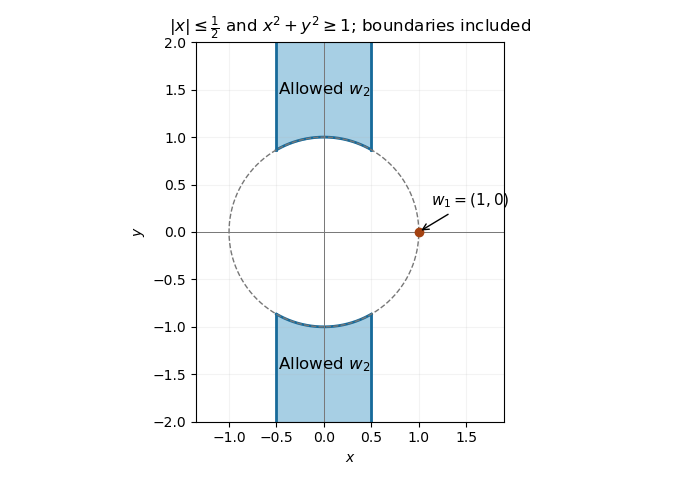
For a second lattice basis, write $v_1=a{w}_1+b{w}_2$, $v_2=c{w}_1+d{w}_2$ with integer coefficients, as just proved. Conversely each $w_i$ is an integer combination of the $v_j$. The change-of-basis matrix $\left(\begin{array}{cc}a& c\\ b& d\end{array}\right)$ and its inverse therefore both have integer entries. Their determinants are integers with product one, giving $\boxed{ad-bc=\pm 1}$. Thus lattice bases are related by a unimodular matrix.