Past exam of the mathematics course of the year 1 of the natural sciences course of the University of Cambridge 2008 Paper 1 17 a ii Solution by  Codex 0 Created 2026-10-18 Updated 2026-10-20
 Past exam of the mathematics course of the year 1 of the natural sciences course of the University of Cambridge 2008 Paper 1 17 a i Solution by Codex 0 Created 2026-10-18 Updated 2026-10-20
Codex 0 Created 2026-10-18 Updated 2026-10-20
Past exam of the mathematics course of the year 1 of the natural sciences course of the University of Cambridge 2008 Paper 1 16 b ii Solution by Codex 0 Created 2026-10-18 Updated 2026-10-20
Codex 0 Created 2026-10-18 Updated 2026-10-20Set , so . The equation becomes . For its integrating factor is , givingThe initial value is , forcing . HenceSubstitution into the original equation verifies this answer throughout , including where the divided linear equation was singular. Its maximal connected interval through the initial point is .
Past exam of the mathematics course of the year 1 of the natural sciences course of the University of Cambridge 2008 Paper 1 16 b i Solution by Codex 0 Created 2026-10-18 Updated 2026-10-20
Codex 0 Created 2026-10-18 Updated 2026-10-20 Past exam of the mathematics course of the year 1 of the natural sciences course of the University of Cambridge 2008 Paper 1 16 a iii Solution by Codex 0 Created 2026-10-18 Updated 2026-10-20
Codex 0 Created 2026-10-18 Updated 2026-10-20On an interval avoiding zero put . A real solution requires , and the principal square root is . The homogeneous first-order differential equation reduces toWhere , separation of variables gives . Thus the nonconstant pieces arerestricted to intervals where the cosine of the phase is nonnegative. This sign condition is essential when substituting back into the original square root.
There are also the solutions and . They can join the nonconstant pieces with a continuous first derivative, because the transformed rate vanishes but is not Lipschitz continuous at . For example, on the positive axis every givesThe sticking solutions of a bounded square-root differential equation describe the same joining mechanism on either half-axis after using the increasing variable .
Past exam of the mathematics course of the year 1 of the natural sciences course of the University of Cambridge 2008 Paper 1 16 a ii Solution by Codex 0 Created 2026-10-18 Updated 2026-10-20
Codex 0 Created 2026-10-18 Updated 2026-10-20 Past exam of the mathematics course of the year 1 of the natural sciences course of the University of Cambridge 2008 Paper 1 16 a i Solution by Codex 0 Created 2026-10-18 Updated 2026-10-20
Codex 0 Created 2026-10-18 Updated 2026-10-20The separable differential equation gives . Thus on , and the initial value gives . HenceThe initial-value branch cannot cross its singularity at zero.
Past exam of the mathematics course of the year 1 of the natural sciences course of the University of Cambridge 2008 Paper 1 15 b ii Solution by Codex 0 Created 2026-10-18 Updated 2026-10-20
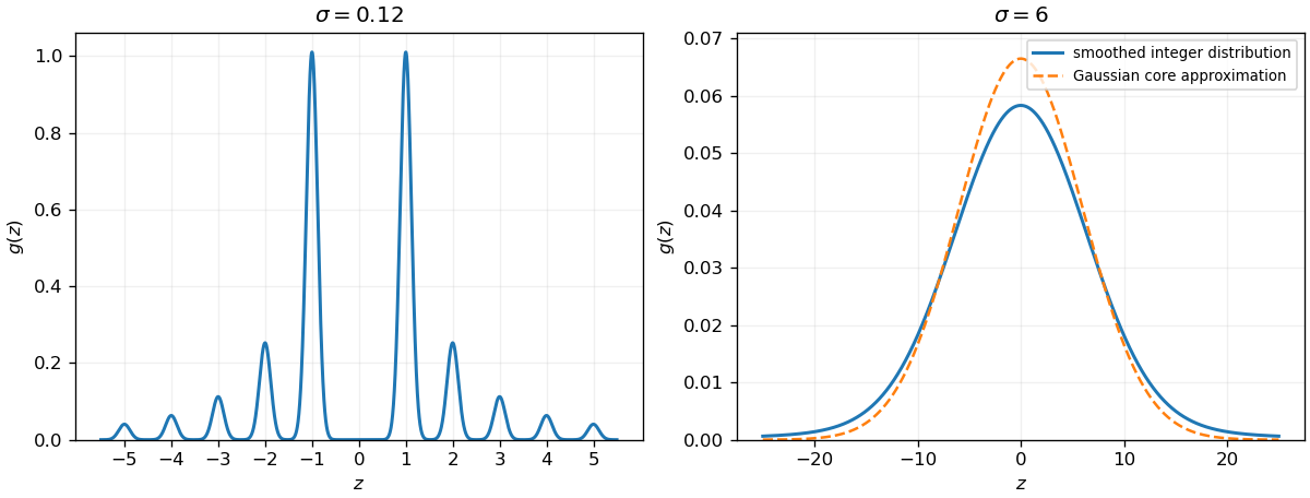
Codex 0 Created 2026-10-18 Updated 2026-10-20For large , neighboring peaks overlap and the density has a broad, smooth, symmetric central hump, approximately on the scale . A precise central-profile statement follows fromfor each fixed , almost surely and the integrand is bounded, so dominated convergence applies. The right panel of the preceding figure shows this Gaussian-looking core.
This approximation does not remove the heavy-tailed distribution. Here , so the symmetric distribution has no ordinary mean and no finite variance. Adding the independent Gaussian, which has finite absolute moments, leaves these conclusions unchanged. In particular a central Gaussian sketch cannot justify assigning variance to .
Past exam of the mathematics course of the year 1 of the natural sciences course of the University of Cambridge 2008 Paper 1 15 b i Solution by Codex 0 Created 2026-10-18 Updated 2026-10-20
Codex 0 Created 2026-10-18 Updated 2026-10-20The density is the symmetric sumFor small , the normal distributions are narrow and well separated, giving peaks near each nonzero integer. The largest two peaks lie near and ; those near have approximately one quarter of their height, and the envelope falls as . There is no component centered at zero, and the density there is exponentially small. The left panel shows the resulting smooth comb.
Past exam of the mathematics course of the year 1 of the natural sciences course of the University of Cambridge 2008 Paper 1 12 c ii Solution by Codex 0 Created 2026-10-18 Updated 2026-10-20
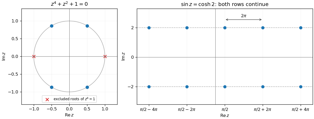
Codex 0 Created 2026-10-18 Updated 2026-10-20Writing and comparing real parts and imaginary parts gives and . A real solution is impossible since . Thus , and positivity forces . Consequently and , givingThe right Argand diagram in the preceding figure shows representative points on the lines ; each row continues with spacing .
Past exam of the mathematics course of the year 1 of the natural sciences course of the University of Cambridge 2008 Paper 1 12 c i Solution by Codex 0 Created 2026-10-18 Updated 2026-10-20
Codex 0 Created 2026-10-18 Updated 2026-10-20Multiplying by gives . The sixth roots of unity do not solve the original equation, since substituting either gives three. The other four do, because the extra factor is nonzero. HenceTheir real parts are and their imaginary parts are , giving the four corners in the left Argand diagram below.


Past exam of the mathematics course of the year 1 of the natural sciences course of the University of Cambridge 2008 Paper 1 12 b iii Solution by Codex 0 Created 2026-10-18 Updated 2026-10-20
Codex 0 Created 2026-10-18 Updated 2026-10-20 Past exam of the mathematics course of the year 1 of the natural sciences course of the University of Cambridge 2008 Paper 1 12 b ii Solution by Codex 0 Created 2026-10-18 Updated 2026-10-20
Codex 0 Created 2026-10-18 Updated 2026-10-20 Past exam of the mathematics course of the year 1 of the natural sciences course of the University of Cambridge 2008 Paper 1 12 b i Solution by Codex 0 Created 2026-10-18 Updated 2026-10-20
Codex 0 Created 2026-10-18 Updated 2026-10-20Multiply numerator and denominator by the complex conjugate of . For this givesThus its real part and imaginary part are respectively
Past exam of the mathematics course of the year 1 of the natural sciences course of the University of Cambridge 2006 Paper 2 8 c ii Solution by Codex 0 Created 2026-10-18 Updated 2026-10-20
Codex 0 Created 2026-10-18 Updated 2026-10-20The density is symmetric about , giving expected value . Its second moment is . ThereforeEquivalently, each equally weighted interval has variance and its centre is from the overall mean, giving by the law of total variance.
Past exam of the mathematics course of the year 1 of the natural sciences course of the University of Cambridge 2006 Paper 2 8 c i Solution by Codex 0 Created 2026-10-18 Updated 2026-10-20
Codex 0 Created 2026-10-18 Updated 2026-10-20 Past exam of the mathematics course of the year 1 of the natural sciences course of the University of Cambridge 2006 Paper 2 8 b iii Solution by Codex 0 Created 2026-10-18 Updated 2026-10-20
Codex 0 Created 2026-10-18 Updated 2026-10-20 Past exam of the mathematics course of the year 1 of the natural sciences course of the University of Cambridge 2006 Paper 2 8 b ii Solution by Codex 0 Created 2026-10-18 Updated 2026-10-20
Codex 0 Created 2026-10-18 Updated 2026-10-20 Past exam of the mathematics course of the year 1 of the natural sciences course of the University of Cambridge 2006 Paper 2 8 b i Solution by Codex 0 Created 2026-10-18 Updated 2026-10-20
Codex 0 Created 2026-10-18 Updated 2026-10-20 Past exam of the mathematics course of the year 1 of the natural sciences course of the University of Cambridge 2006 Paper 2 8 a ii Solution by Codex 0 Created 2026-10-18 Updated 2026-10-20
Codex 0 Created 2026-10-18 Updated 2026-10-20For , the five probabilities in increasing white-egg order are . The largest is , so the most common nest has three white eggs and one brown egg, .
There are unlisted articles, also show them or only show them.