Past exam of the mathematics course of the University of Cambridge 2008 ii Paper 2 14C ii Solution by  Codex 0 Created 2026-09-24 Updated 2026-10-14
There is a branch-phase discrepancy in the printed identity. Set using the positive real base. Shrink the anticlockwise loop at . The outward interval carries phase and its return phase ; their difference gives . The clockwise loop at starts with phase and returns with , giving the same coefficient on . Small endpoint circles vanish for . Thus the branch phase in a figure-eight analytic continuation integral isIf the printed interval integral uses the prescribed argument , then , and the corrected formula is insteadFor example at , , and ; the printed right side without the phase would be the real number . Interpreting its interval integrand as restores the intended identity.
On the fixed contour away from its branch points, the continued logarithm is bounded and is entire in , uniformly on compact sets. Hence is an entire function. Division by the sine gives a meromorphic continuation of , and multiplication by gives the continuation of the specified . The only candidate singularities are integers, at most simple. All are removable because the interval integral is already holomorphic on .
The negative integers , , are genuine simple poles. At such a point the contour integrand is single-valued andThe first residue is times a rational number. The second is times a nonzero rational number: expand at , whose degree- coefficient has sign and nonzero magnitude. They cannot be equal because is irrational. Therefore , and the simple sine zero creates a simple pole. In particular .
A circle enclosing both branch points has total logarithmic change , rather than zero as for the figure eight. For a circle based at with initial real logarithm, shrinking it leaves a connector from to as well as the two banks of the interval. Explicitly its integral isThus it is not just a known sine factor times : an additional endpoint-singular integral remains. The figure-eight contour eliminates precisely that connector term. This explains why replacing it by the large circle does not give the same direct continuation method.
Past exam of the mathematics course of the University of Cambridge 2008 ii Paper 2 14C i Solution by Codex 0 Created 2026-09-24 Updated 2026-10-14
Codex 0 Created 2026-09-24 Updated 2026-10-14Parametrize the continued branch by , . Then , givingThe apparent singularity at zero is removable, so is an entire function. The factor shows its dependence on the contour radius; for instance . The integrand is continued along the contour and generally returns on a different branch, so this is not an ordinary integral of a single-valued holomorphic function around a closed loop.
Past exam of the mathematics course of the University of Cambridge 2008 ii Paper 2 13B c Solution by Codex 0 Created 2026-09-24 Updated 2026-10-14
Codex 0 Created 2026-09-24 Updated 2026-10-14A travelling wave obeys , so the mechanical potential in the requested form is , up to an additive constant. HereIts stationary points are maxima at and a minimum at . Since and , the two maxima have equal height at ; the maximum at is lower for and higher for .
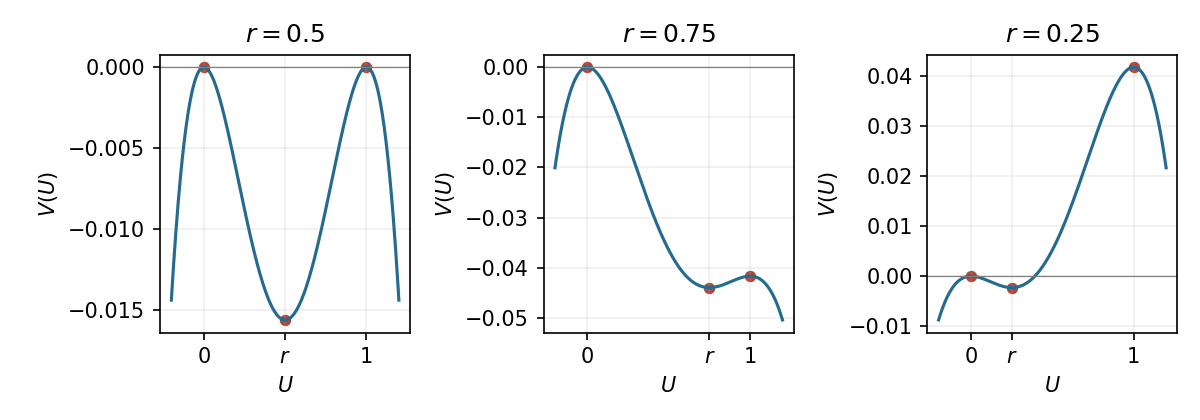

Multiply the wave equation by and integrate along the heteroclinic orbit. The endpoint derivatives vanish, and , , soConsequentlyThe integral is positive for a nonconstant front. In fact substitution of the same logistic shape from part (b) gives the exact velocity . Thus the phase invades rightwards when , the zero phase invades leftwards when , and the balanced front is stationary.
Past exam of the mathematics course of the University of Cambridge 2008 ii Paper 2 13B b Solution by Codex 0 Created 2026-09-24 Updated 2026-10-14
Codex 0 Created 2026-09-24 Updated 2026-10-14At , write , so . Multiplying the stationary equation by gives . The endpoint values and vanishing endpoint derivatives make . For the decreasing connection,Separate variables and absorb the integration constant into a translation . The logistic front of a bistable cubic equation isIt approaches on the left and on the right and satisfies the stationary differential equation directly.
Past exam of the mathematics course of the University of Cambridge 2008 ii Paper 2 13B a Solution by Codex 0 Created 2026-09-24 Updated 2026-10-14
Codex 0 Created 2026-09-24 Updated 2026-10-14For spatially homogeneous solutions, the bistable cubic reaction-diffusion equation reduces to . Its equilibria are , andThus and are asymptotically stable, while is unstable. Small spatial Fourier perturbations have growth rates , so diffusion also leaves the two outer uniform states linearly stable.
Past exam of the mathematics course of the University of Cambridge 2008 ii Paper 1 7A i Solution by Codex 0 Created 2026-09-24 Updated 2026-10-14
Codex 0 Created 2026-09-24 Updated 2026-10-14For , the first integralhas . The equilibrium points are and . The linearization has eigenvalues at the origin and at . The origin is a center equilibrium: the sufficiently small positive level sets of are closed curves, since its Hessian matrix there is positive-definite. The other equilibrium is a saddle equilibrium.
At the saddle, , and the separatrix satisfiesIts two branches with form a homoclinic orbit through the saddle; its remaining branches extend to . Inside the loop, the closed trajectories run clockwise: above the horizontal axis . The saddle directions have slopes and . Outside the loop there are unbounded trajectories. The left panel shows the closed orbits and all saddle branches.
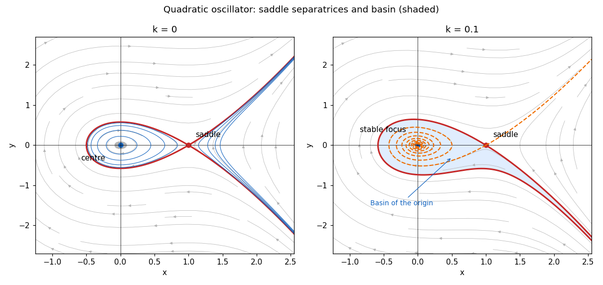
Conservative phase portrait and the attracting basin after adding weak damping
. Details. 
Past exam of the mathematics course of the University of Cambridge 2008 ii Paper 1 38C b Solution by Codex 0 Created 2026-09-24 Updated 2026-10-14
Codex 0 Created 2026-09-24 Updated 2026-10-14For a linear system write , where is the diagonal. The Jacobi method iteratesHere , and has nonnegative off-diagonal entries with row sums at most one. Rows adjacent to the boundary have sum strictly less than one; those at purely interior stencil vertices have sum one. Thus .
To prove strict spectral radius below one, suppose with , and choose an index with . Inequality forces that row sum to equal one and every linked neighbor to attain the same maximum modulus. Propagate this along the connected axial grid to a boundary-adjacent row, whose row sum is strictly less than one, a contradiction. All eigenvalues therefore have modulus strictly below one. Hence and the Jacobi errors tend to zero from every initial vector. The unique solution exists by positive definiteness, so
Past exam of the mathematics course of the University of Cambridge 2008 ii Paper 1 38C a Solution by Codex 0 Created 2026-09-24 Updated 2026-10-14
Codex 0 Created 2026-09-24 Updated 2026-10-14Number the interior grid vertices in any order. The diagonal of is , and off-diagonal weights are for axial neighbors and for diagonal neighbors. Each link weight is symmetric, so is symmetric. Extend the interior grid values by zero to the boundary. Since the eight stencil weights sum to , grouping links giveswhere or and each interior link is counted once. Every term is nonnegative. If the quadratic form vanishes, neighboring interior values agree, and every vertex linked to the boundary has value zero. The axial-link grid is connected and reaches the boundary, so all values are zero. Thus . Reordering vertices replaces by for a permutation matrix , preserving both properties.
Past exam of the mathematics course of the University of Cambridge 2008 ii Paper 1 36A b Solution by Codex 0 Created 2026-09-24 Updated 2026-10-14
Codex 0 Created 2026-09-24 Updated 2026-10-14Integrating the velocity profiles over their respective half-channels gives volume flux per unit widthWith , the requested ratio isAt , both fluxes equal and the ratio is one. For , , and the ratio is asymptotic to , tending to zero. The lower fluid flows between the wall and an interface which becomes effectively stationary; the upper fluid carries vanishing flux despite finite limiting stress.
Past exam of the mathematics course of the University of Cambridge 2008 ii Paper 1 36A a Solution by Codex 0 Created 2026-09-24 Updated 2026-10-14
Codex 0 Created 2026-09-24 Updated 2026-10-14The signed tangential stress component is . ThusWhen , these approach and , the usual symmetric plane Poiseuille flow stresses. When , they approach and . The upper fluid's velocity tends to zero, but its viscosity times velocity gradient has a finite limit. These are tensor components; traction on a chosen wall normal includes that normal's sign.
Past exam of the mathematics course of the University of Cambridge 2008 ii Paper 1 32D b Solution by Codex 0 Created 2026-09-24 Updated 2026-10-14
Codex 0 Created 2026-09-24 Updated 2026-10-14The spatial translation operator is . From and the preceding central-commutator result,Thus , consistent with . Since , the translated wavefunction is .
For the quantum harmonic oscillator, the creation and annihilation operators give . Put . The central commutator of and is , soAs and ,Taking position wavefunctions provesThe coefficient squares sum to , checking normalization of this coherent state.
Past exam of the mathematics course of the University of Cambridge 2008 ii Paper 1 32D a Solution by Codex 0 Created 2026-09-24 Updated 2026-10-14
Codex 0 Created 2026-09-24 Updated 2026-10-14Write , so . Repeated use of the product rule for the commutator gives . Summing the exponential series yieldsThese manipulations hold for bounded operators, or as identities on a common invariant domain where the series and derivatives are justified.
The same commutation relation implies : its derivative is and its initial value is . Put . ThenFor the specified , the operator commutes with . Indeed conjugation by sends to , and subsequent conjugation by restores . Thereforeso . At this proves the central-commutator case of the Baker--Campbell--Hausdorff formula:The last equality holds because commutes with .
Past exam of the mathematics course of the University of Cambridge 2008 ii Paper 1 29C iii Solution by Codex 0 Created 2026-09-24 Updated 2026-10-14
Codex 0 Created 2026-09-24 Updated 2026-10-14Start a characteristic curve at with . The Characteristic curve equations give , , , so . Therefore the two branches areEach is on . The plus branch matches for , whereas the minus branch matches it for . Differentiating gives and , verifying wherever .
On the initial line, the normal Characteristic curve speed is , nonzero away from the origin. Thus the local existence theorem gives precisely these separate local branches near positive and negative initial points. At the branches merge and their derivatives become singular. There is no solution realizing the entire initial line in a neighborhood of the origin: the data force , while the equation and force . The failure at this Characteristic curve point is a genuine limitation of the printed global initial-data request.
Past exam of the mathematics course of the University of Cambridge 2008 ii Paper 1 29C ii Solution by Codex 0 Created 2026-09-24 Updated 2026-10-14
Codex 0 Created 2026-09-24 Updated 2026-10-14Here the characteristic curves are straight lines , , along which . If , every nearby point determines a unique starting point and travel parameter:Integrating along the Characteristic curve givesThe non-characteristic condition is exactly what permits division by and ensures transversality to the data hyperplane. If , the Characteristic curve lines starting there never leave it. Moreover the prescribed data must satisfy on the hyperplane even to be compatible. If they do, the Characteristic curve construction still leaves off-hyperplane data undetermined; if they do not, no solution exists.
Past exam of the mathematics course of the University of Cambridge 2008 ii Paper 1 29C i Solution by Codex 0 Created 2026-09-24 Updated 2026-10-14
Codex 0 Created 2026-09-24 Updated 2026-10-14For a first-order quasilinear partial differential equation, take coefficients , prescribed data on a smooth hypersurface , and a point . The data are non-characteristic there ifwhere is any nonzero normal to . Then there is a neighborhood of on which a unique solution realizes the data. Uniqueness is local, after restricting to a neighborhood swept out by the nearby characteristics.
The method of characteristics solves , from points of . In local surface coordinates , the map has nonsingular derivative at exactly under the stated normal condition. The inverse function theorem makes these variables local coordinates, giving the asserted solution and uniqueness.
Past exam of the mathematics course of the University of Cambridge 2008 ii Paper 1 28J e Solution by Codex 0 Created 2026-09-24 Updated 2026-10-14
Codex 0 Created 2026-09-24 Updated 2026-10-14The Black-Scholes implied volatility of a traded call price is the volatility which makes the Black-Scholes formula equal to . Forthe price is a continuous strictly increasing function of , by its positive vega, with precisely these endpoint limits. The intermediate value theorem and strict monotonicity therefore give a unique positive implied volatility. The lower endpoint corresponds to the limiting value ; the upper endpoint is reached only as . Prices outside the bounds admit the arbitrages above and have no implied volatility.
Past exam of the mathematics course of the University of Cambridge 2008 ii Paper 1 28J d Solution by Codex 0 Created 2026-09-24 Updated 2026-10-14
Codex 0 Created 2026-09-24 Updated 2026-10-14Write for the standard normal density. Differentiating the Black-Scholes formula and using givesThe last equality follows by differentiating . This derivative is the option's vega.
Past exam of the mathematics course of the University of Cambridge 2008 ii Paper 1 28J c Solution by Codex 0 Created 2026-09-24 Updated 2026-10-14
Codex 0 Created 2026-09-24 Updated 2026-10-14As , the Black-Scholes formula tends to . This also follows by discounting the deterministic zero-volatility payoff; at equality the limiting value is zero.
If and a call trades at , buy a call, short one share, and buy a bond paying at maturity. Invest the positive initial surplus . At maturity the call, share and bond together pay , in addition to the strictly positive invested surplus. If the lower bound is zero, violating it means : buy the call and invest the cash received, obtaining a nonnegative option payoff and a strictly positive bank payoff. Both strategies are arbitrages.
Past exam of the mathematics course of the University of Cambridge 2008 ii Paper 1 28J b Solution by Codex 0 Created 2026-09-24 Updated 2026-10-14
Codex 0 Created 2026-09-24 Updated 2026-10-14 Past exam of the mathematics course of the University of Cambridge 2008 ii Paper 1 28J a Solution by Codex 0 Created 2026-09-24 Updated 2026-10-14
Codex 0 Created 2026-09-24 Updated 2026-10-14For positive , the Black-Scholes formula usesTo hedge the sold European call option, buy shares and borrow in cash. This long replicating strategy has initial value , financed by the option premium. The share holding must subsequently be rebalanced according to the option's option delta in a self-financing strategy.
There are unlisted articles, also show them or only show them.