The Jacobi method solves a linear system by updating every coordinate from the same old vector. It requires every diagonal entry to be nonzero. Isolating coordinate in row gives the simultaneous ruleHere is the iteration matrix. A sweep computes a complete new vector before replacing the old one, so its coordinate updates can run independently.[ref]
Notes for Ma221 Lecture 21, Nov 10 2009. Math 221, Matrix Computations, Fall 2009; Jacobi: component loop and splitting immediately before Gauss-Seidel
For a sparse matrix, a sweep needs work proportional to the stored nonzero entries, while Gaussian elimination may create fill-in. The Jacobi method is therefore a simple starting point for large linear systems, and the weighted Jacobi method supplies a useful building block of a multigrid method. Its beauty is that a local row correction becomes a global eigenvalue question: the convergence criterion for a stationary iteration is exactly .
Consider the original linear system with a symmetric matrix that is also a tridiagonal matrix:Here and the Jacobi method readsStarting from , the first three vectors areEvery right-hand side uses superscript , including the middle row, even when a new first coordinate has already been computed.
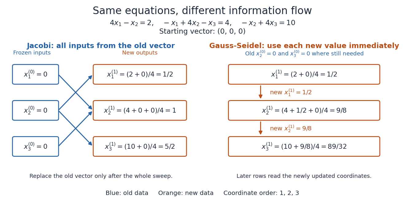
Simultaneous old-to-new component updates in the Jacobi method, compared with immediate reuse in the Gauss-Seidel method
. Details. For comparison, a first Gauss-Seidel method sweep in coordinate order givesThe new first coordinate enters the middle update, and the new second coordinate enters the final update. Accidentally overwriting old coordinates during a Jacobi method sweep therefore changes the mathematical method.
For the Jacobi iteration for a three-variable tridiagonal system,An orthonormal eigenbasis iswith eigenvalues , , and , respectively. These are error modes: their shapes persist under the iteration matrix, while their coefficients change. Direct multiplication verifies them, or expansion of the determinant gives . Thus and convergence holds for every starting vector.
With , the initial forward error has coefficientsFor ,The zero mode disappears after one sweep; the negative mode alternates in sign. The Euclidean norm drops by exactly per sweep from onward. The first norm drop is different because includes the zero mode. A starting error proportional to would disappear entirely in one sweep, faster than the spectral radius predicts for generic errors.
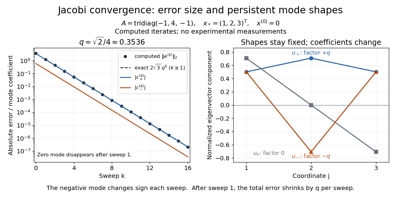
Computed Jacobi method error curves and eigenvector modes for the original three-variable tridiagonal matrix
. Details. The curves are computed iterates and exact formulas for this linear system. Since , the same eigenvectors have eigenvalues , , and for . They prove that is a positive-definite matrix, and give the condition number used in residual and forward error in a stationary iteration.
A strictly diagonally dominant matrix guarantees convergence of the Jacobi method for every initial vector.[ref]
Notes for Ma221 Lecture 21, Nov 10 2009. Math 221, Matrix Computations, Fall 2009; Theorem 1 on strict row diagonal dominance and its proof beginning “Split A = D − (D − A)”
Indeed, using the maximum norm , the induced operator norm is the largest absolute row sum. The Jacobi method has and for , soThis gives a cheap sufficient check without computing any eigenvalues. For the Jacobi iteration for a three-variable tridiagonal system, the absolute row sums of are , giving . The true spectral radius gives a sharper eventual rate.
Strict diagonal dominance is sufficient, not necessary: violates it in the first row, but its Jacobi method has eigenvalues and converges. Conversely, being a positive-definite matrix alone is insufficient: the Jacobi convergence for a three-by-three equicorrelation matrix with has positive eigenvalues for , but spectral radius for its iteration matrix. The extra tridiagonal matrix structure in Jacobi convergence for a symmetric positive-definite tridiagonal matrix is therefore substantive.
For , with the four-dimensional unit superdiagonal, the Jacobi method has eigenvalues , . The Gauss-Seidel method has two zero eigenvalues and . Therefore both methods converge for every starting vector exactly when . This equality of convergence ranges follows from their spectra, not from positive-definiteness of the nonsymmetric coefficient matrix.
Equivalently, the weighted Jacobi method takes a weighted average of the old vector and its full Jacobi method update: . If , its iteration matrix multiplies that eigenvector by . For the diagonal-4 Jacobi iteration for a three-variable tridiagonal system, the factors are and ; a Poisson equation smoothing parameter must not be inferred from this different matrix.
For the five-point discretization of on the unit square, the weighted iteration eigenvalues are . A fixed parameter converges for every mesh when , but poorly damps the highest frequencies.
For the five-point Dirichlet Poisson matrix, weighted Jacobi iteration has sine-mode multiplier . Call a mode high-frequency if at least one cosine is nonpositive. Then the sum lies in , so for the multiplier lies in . This uniform damping makes the iteration a useful smoother for a multigrid method, even though low-frequency multipliers approach one on fine grids. Balancing and shows why is the minimax parameter for this high-frequency interval. The two-dimensional high-frequency set gives a different optimum from the familiar one-dimensional value .
For the centered second-difference matrix with diagonal and off-diagonals , the weighted-Jacobi eigenvalues areThe method converges for every grid size exactly when .
Multiplying both and by leaves and the weighted Jacobi method unchanged. Thus the same formula applies to the positive second-difference matrix with diagonal and neighboring entries , the finite difference form of the one-dimensional Poisson equation with Dirichlet boundary conditions. Its eigenvectors have components , and has eigenvalues . At , upper-half modes have factors between and , while low-frequency factors remain close to one on fine grids. This explains why the weighted Jacobi method helps a multigrid method by reducing oscillatory errors, even when it is a slow solver on its own.[ref]
CS267: Supplemental Notes for Lecture 17 — How Multigrid Damps High Frequencies by James Demmel. Error eigenvector expansion, coefficient 1/3 + (2/3) cos(jπ/2^i), and concluding upper-half-frequency attenuation statement
For the one-dimensional Dirichlet second-difference grid, high sine modes have eigenvalues , with and . Let and be the smallest and largest of these . Convexity gives attenuation . Balancing its endpoint values with opposite signs gives the displayed exact minimax choice. For odd , ; for even , , and always . Only in the large-grid or uniform-in-grid limit do these become , .
For a three-by-three matrix with diagonal entries one and every off-diagonal entry , the Jacobi method iteration matrix has eigenvalue on the all-ones vector and eigenvalue with multiplicity two on its orthogonal complement. Its spectral radius is , so Jacobi iteration converges exactly when .
If is symmetric positive definite and tridiagonal, set . Thenis positive definite. Applying the Householder-John theorem to and proves that the Jacobi iteration converges.
Articles by others on the same topic



The Jacobi method is an iterative algorithm used to solve systems of linear equations. It is particularly useful for large sparse systems, where the matrix involved has a significant number of zero elements. The method is named after the German mathematician Carl Gustav Jacob Jacobi.