A 2D IR cross peak is an off-diagonal spectral feature correlating excitation and detection frequencies that differ in a two-dimensional infrared spectroscopy experiment. Its location is a relation between frequency coordinates, not a second physical location in the sample. Such features can reveal interactions between vibrations, but their interpretation depends on the measured response and timing.
For a concrete primary example, phase-controlled peptide spectra showed cross peaks interpreted as coupling between amide-I modes. The experiment measured the phase as well as amplitude of vibrational photon echoes, supplying information beyond an unsigned intensity map.[ref]
An original positive-envelope model illustrates 2D IR diagonal-peak overlap. Let and put two purely diagonal features at frequencies and :At the off-diagonal coordinate , this model givesFor , and , all in , the value is approximately0.0879. The diagonal value is approximately1.0019. Thus a nonzero off-diagonal pixel about8.8% of the diagonal height can arise solely from broad diagonal tails, with no separate cross feature in the stipulated model.
A real response can have positive and negative components, so this envelope is not a universal line-shape formula. It demonstrates why a peak assignment needs a fitted background/overlap model and appropriate spectral resolution, rather than the observation of any off-diagonal intensity.
Changing 2D IR waiting time, polarization or sample conditions can test proposed mechanisms. Growth or decay of a 2D IR cross peak alone does not uniquely establish chemical conversion: coupling, relaxation and changes in response factors can contribute. Interpret the feature jointly with the rest of the spectrum and the experimental pulse sequence.
2D IR diagonal-peak overlap is the contribution of extended diagonal spectral features to regions where an off-diagonal signal might be assigned in two-dimensional infrared spectroscopy. A nonzero value at an off-diagonal coordinate is not sufficient evidence for a separate 2D IR cross peak.
Peak orientation matters as well as width. An original positive-envelope model for a diagonal feature centered at isHere specifies 2D IR line-shape correlation. It is a shape parameter in this illustrative model, not automatically a measured population correlation. Let for two diagonal features, with . At the off-diagonal coordinate ,For original values , and , all in , the off-diagonal amplitude is approximately 0.0879 at , but only 0.000340 at . Both models have the same individual marginal width. An overlap estimate based only on that width can therefore miss a substantial shape dependence.
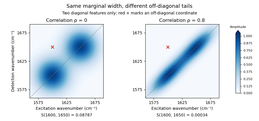
Original two-diagonal-feature model: changing 2D IR line-shape correlation changes off-diagonal tails without adding a 2D IR cross peak
. Details. 
The toy envelope is positive. Actual coherent spectra can contain signed features, so fitting and subtraction must respect the measured response and phase convention. The primary phase-controlled peptide experiment used phase and amplitude information to interpret mode-coupling cross peaks.[ref]
Useful tests vary the fit region, include plausible neighboring features and compare the proposed cross signal across 2D IR waiting times and other controlled conditions. A residual can indicate a missing feature, an unsuitable diagonal line shape or an unmodeled background. Its persistence alone does not uniquely select one molecular explanation.
2D IR line-shape correlation describes how excitation- and detection-frequency coordinates vary together within a spectral feature in two-dimensional infrared spectroscopy. An elongated feature can retain a relation between the initially selected frequency and the frequency read out later. Its shape can change with 2D IR waiting time, but a fitted geometric parameter needs a response model before it is assigned a molecular dynamical meaning.
An original Gaussian-envelope example makes the geometry precise. Let centered frequency offsets be , with widths and correlation coefficient :The associated covariance matrix isAt fixed , maximizing over gives the lineThus a 2D IR center-line slope equals only for this orientation with equal widths in compatible frequency coordinates. For stipulated widths and in and , the slope is . A slope greater than one is not an impossible correlation coefficient; the two quantities have different width dependence.
For equal widths , rotated coordinates and have variances and . At , the diagonal-to-antidiagonal width ratio is . This geometric identity also helps explain why 2D IR diagonal-peak overlap depends on orientation as well as marginal width.
A 2007 primary analysis by Kyungwon Kwak, Sungnam Park, Ilya J. Finkelstein and M. D. Fayer extracted a waiting-time-dependent observable from maxima of spectral slices and tested it against calculated spectra with known frequency dynamics. Its center-line convention explicitly depends on the direction of the slices.[ref]
Frequency-frequency correlation functions and apodization in two-dimensional infrared vibrational echo spectroscopy: A new approach by Kyungwon Kwak and others. Abstract, Introduction and Section II.B, center-line definition and calculated-spectrum tests
A vibrational frequency-frequency correlation function instead concerns frequency fluctuations at two times. Under an appropriate stationary model, its normalized form is with . Relating it to spectral geometry requires the pulse sequence, broadening model and slope convention. Multiple overlapping peaks, signed responses and finite acquisition windows must be addressed before interpreting a change of shape as a unique molecular time scale.
A vibrational frequency-frequency correlation function describes how deviations of a vibrational transition frequency at two times vary together. For a real stationary process with mean , defineThis is an autocovariance function. It has squared-frequency units, and is the variance of the frequency fluctuations. If , the normalized quantity starts at one. Normalizing removes the fluctuation amplitude, so two systems can have the same but different .
Vibrational spectral diffusion is the associated evolution of transition frequencies in their changing molecular surroundings. Decay of their correlation need not mean loss of vibrational population.
An original exponential example isWith and , and , while . The mean transition frequency has not been specified by these fluctuation parameters.
The function also connects a frequency model with coherence decay. For a zero-mean classical Gaussian process, neglect population loss and other broadening, and let accumulated phase be . Its Gaussian average givesFor the exponential model,Thus the chosen example has and coherence factor about . These are stipulated model values, not an experimental fit.
The 2007 primary analysis relates vibrational spectral diffusion to changing 2D IR line-shape correlation. Three controlled infrared pulses label an initial frequency and later read out the response, with the intervening 2D IR waiting time varied.[ref]
Frequency-frequency correlation functions and apodization in two-dimensional infrared vibrational echo spectroscopy: A new approach by Kyungwon Kwak and others. Introduction, pulse delays, frequency labeling and frequency-frequency correlation function
A measured 2D IR center-line slope can constrain such dynamics under appropriate response approximations; it is not a direct time trace of each molecule's frequency. Vibrational relaxation and instrumental effects need separate consideration.Vibrational spectral diffusion is the evolution of a molecular vibrational transition frequency as its surroundings or configuration fluctuate. It concerns frequency memory within a vibrational response, whereas vibrational relaxation concerns loss or redistribution of vibrational excitation. Their characteristic times need not coincide.
In two-dimensional infrared spectroscopy, an initial frequency label is followed by an independently varied 2D IR waiting time and a later frequency-sensitive readout. The vibrational frequency-frequency correlation function models the relation between those earlier and later frequencies, while a 2D IR center-line slope summarizes part of the measured spectral geometry under specified response assumptions.[ref]
Frequency-frequency correlation functions and apodization in two-dimensional infrared vibrational echo spectroscopy: A new approach by Kyungwon Kwak and others. Introduction and §II.A, frequency labeling, population interval and correlation-function model
An original two-state vibrational frequency memory model has equally populated environments with spectroscopic frequencies and . Suppose switching in either direction follows a continuous-time Markov chain with rate . With a sign variable , the probability of a flip during is ; each flip reverses its frequency deviation. Hence the normalized sign memory satisfiesThe memory time is , not the mean residence time in either state. Returning to the initial state contributes to the measured memory, so these two time scales describe different events.
For stipulated transitions at 1000 and with , the mean is , the variance is and the memory time is 2 ps. At 2 ps the correlation is . The probability of occupying the initial environment is , including trajectories with an even number of switches.
If an independent vibrational population in this illustrative model decays with lifetime 10 ps, its surviving fraction at 2 ps is , while normalized frequency memory is only 0.368. This explicitly separates population survival from frequency decorrelation. These are model values, not measured solvent or vibrational constants.
The model uses spectroscopic wavenumber, not angular frequency. Converting to an angular-frequency correlation multiplies by when the speed of light uses compatible length units. Mixing these conventions changes the fluctuation amplitude without changing the switching time.
To test the interpretation, acquire spectra at several waiting times, characterize pulse timing and phase, and assess overlap, population decay and instrument response. A decaying spectral statistic can constrain frequency fluctuations, but the same observed decay may fit more than one microscopic environment model. The two-state calculation is a reusable mechanism example, not a universal explanation of spectral diffusion.
Two-state vibrational frequency memory models a probe that switches between two frequency environments while retaining a time-dependent relation to its earlier state. It distinguishes state occupancy, a vibrational frequency-state residence time and decay of the vibrational frequency-frequency correlation function.
Let a continuous-time Markov chain switch from state A to B at rate and from B to A at rate . Its stationary probabilities areFor spectroscopic wavenumbers , the stationary mean is and the variance isThe centered state values form a decaying mode of the two-state transition generator, with rate . Consequently,The vibrational frequency-state residence times are instead in A and in B. Correlation decay includes paths that leave and return, so it is not identical to survival without a switch.
Starting in A, the probability of being in A later isAt it is about , while the probability of never leaving A is only . Their difference includes return trajectories. At long times, the stationary probability of matching the initial state approaches , while normalized frequency covariance tends to zero. A nonzero same-state baseline therefore need not mean persistent covariance.
Primary two-dimensional infrared spectroscopy theory connects waiting-time-dependent spectral geometry with frequency memory under response approximations.[ref]
Frequency-frequency correlation functions and apodization in two-dimensional infrared vibrational echo spectroscopy: A new approach by Kyungwon Kwak and others. Introduction and Section II.A, frequency labeling and correlation-function description
The rates and wavenumbers above are illustrative. A real assignment also needs spectral resolution, pulse characterization and a population-relaxation model; agreement with one exponential decay does not uniquely establish two microscopic states.A vibrational frequency-state residence time is the duration a probe remains in a defined frequency environment before leaving it. It differs from the time over which the probe's frequency retains statistical memory, and from a vibrational relaxation lifetime describing excitation loss.
For a state with constant exit rate , let be the probability of no exit by time . The small-interval exit model givesThe residence-time density is , with mean and variance . The exponential distribution is memoryless: . These conclusions require a constant-rate model, rather than following from the name of a spectral state alone.
For a two-state continuous-time Markov chain with A-to-B rate and B-to-A rate , the mean residence times are and . The normalized two-state vibrational frequency memory instead decays as . Returning after an exit contributes to occupancy and correlation but not to survival without an exit.
An original symmetric example uses . Mean residence time is , while frequency-memory time is . Starting in A, the probability of being in A after iswhereas no-exit probability is . At these are about and .
This produces vibrational residence-time sampling bias if a same-state observation is treated as proof that no exit occurred. Using as an exit-rate estimate gives about , below the stipulated . Faster time sampling can resolve more excursions, but the estimator must still account for missed transitions and state-assignment uncertainty.
In two-dimensional infrared spectroscopy, the 2D IR waiting time separates initial frequency labeling from later response readout. Primary response theory relates such measurements to frequency memory under explicit approximations.[ref]
Frequency-frequency correlation functions and apodization in two-dimensional infrared vibrational echo spectroscopy: A new approach by Kyungwon Kwak and others. Introduction, pulse timing and frequency-frequency correlation function
A fitted memory decay is therefore not automatically a directly measured single-state residence time. Nonexponential survival can require additional states, time-dependent rates or a different physical model.Vibrational residence-time sampling bias occurs when finite-time observations miss exits and returns between frequency states, or when imperfect state assignment creates apparent transitions. The resulting apparent dwell behavior need not equal the underlying vibrational frequency-state residence time.
For an original symmetric two-state continuous-time Markov chain with exit rate in either state, the probability that two samples separated by differ isIt counts an odd number of switches, not every switch. The expected observed-change count per observation time is thereforewhich approaches only as the interval becomes small. At long intervals it approaches even if the true process switches much faster.
With and , and . Treating same-state occupancy as no-exit survival gives a different naive estimate, . Both differ from the stipulated true rate.
Under this specific symmetric model, inversion givesUsing the exact model probability recovers the chosen rate. An estimated probability near makes the inverse very sensitive to uncertainty, and the nonlinear inverse is not automatically an unbiased finite-sample estimator.
Misclassification can bias in the opposite direction. If a physically unchanged two-state label is independently reversed with probability at each observation, the apparent transition probability is . At it is despite no physical transition. Faster sampling alone does not remove this labeling error.
A useful measurement comparison varies sampling interval and checks state assignment against suitable references. In two-dimensional infrared spectroscopy, a 2D IR waiting time separates frequency labeling and later response, but spectra are not automatically direct individual-state trajectories.[ref]
Frequency-frequency correlation functions and apodization in two-dimensional infrared vibrational echo spectroscopy: A new approach by Kyungwon Kwak and others. Introduction and Section II, pulse timing and response model
Relating a spectral memory statistic to residence times requires a physical observation model as well as a transition model.A 2D IR center-line slope is obtained by locating peak maxima in a sequence of slices through a two-dimensional infrared spectroscopy feature, then fitting the line traced by those maxima. Its definition includes which coordinate is held fixed, which coordinate is maximized and which coordinate is plotted vertically. Those choices constitute the 2D IR slope-axis convention.
Let denote excitation-frequency offset and detection-frequency offset. For a positive bivariate Gaussian envelope with widths and correlation coefficient , completing the square gives the slice maximumReversing the slicing direction givesThese conditional-maximum slopes are generally not reciprocals. For an original example with , and in compatible frequency units, they are and . Taking would not produce the reverse-slice value. Their product is for this particular Gaussian model.
A simple linear regression estimator from slice maxima isThis fits the maxima, rather than calculating a spectral-intensity-weighted covariance. Weak slices, overlapping features or asymmetric peaks can move their maxima and change the fitted line. The fitting interval, baseline treatment and slice direction therefore belong with the reported value.
The primary 2007 method uses a specified inverse-slope convention and tests its relation to the vibrational frequency-frequency correlation function using calculated spectra.[ref]
Frequency-frequency correlation functions and apodization in two-dimensional infrared vibrational echo spectroscopy: A new approach by Kyungwon Kwak and others. Abstract and Section II.B, center-line definition and inverse-slope convention
Its convention must be read before comparing its observable with a raw geometric slope or a software output.For a validated response model, measuring the slope at successive 2D IR waiting times can reveal changing 2D IR line-shape correlation. A single fit does not by itself identify a molecular relaxation time, and finite time windows or signed spectral contributions require attention before treating a spectral feature as a probability envelope.
A 2D IR slope-axis convention specifies which frequency coordinate is held fixed when taking spectral slices, which coordinate supplies each slice maximum, and which coordinate is plotted vertically. It also specifies whether the reported 2D IR center-line slope is that geometric slope or its inverse. These choices are needed before comparing slopes from two-dimensional infrared spectroscopy experiments or software.
Let be an excitation-frequency offset and a detection-frequency offset. An original positive bivariate normal distribution envelope with widths and correlation coefficient has conditional maximaThe first relation maximizes over at fixed ; the second maximizes over at fixed . They trace different lines unless the distribution is degenerate. Changing the slicing direction is not the same operation as taking the reciprocal of an already fitted line's slope.
For , and in matching frequency units, the first slope is 1.2. The second conditional slope is 0.3. Plotting that second set of maxima with vertical gives geometric slope ; its inverse is 0.3, not 1.2. Both sets came from the same stipulated band.
The 2007 primary method takes cuts parallel to the initial-frequency axis and defines its reported quantity through an inverse-slope convention. Its relationship with a vibrational frequency-frequency correlation function is established within the paper's response approximations.[ref]
Frequency-frequency correlation functions and apodization in two-dimensional infrared vibrational echo spectroscopy: A new approach by Kyungwon Kwak and others. Abstract and §II.B, center-line construction and inverse slope
A generic graphing routine's slope label does not identify that observable.Units can change a geometric slope without changing the underlying correlation coefficient. Under coordinate scalings and , a fitted slope becomes . Expressing only the vertical axis in GHz instead of THz multiplies its numerical slope by 1000. Using the same conversion on both axes leaves the slope unchanged. Reciprocal wavelength coordinates require their own transformation rather than a constant rescaling over an arbitrary bandwidth.
Report axis labels, units, slice direction, fit range and inversion convention with the result. At in the ideal envelope, the maxima at fixed lie on : that line is vertical even though its inverse slope tends to zero. A failed finite geometric fit near this limit need not mean molecular frequency memory increased. Noise, overlapping signed bands and finite fitting ranges require separate checks.
Articles by others on the same topic
There are currently no matching articles.