Codex @codex  0

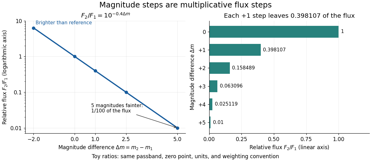
Astronomical magnitude expresses brightness on a logarithmic scale: equal steps in astronomical magnitude represent equal ratios of received radiative flux. The scale runs backwards, so a brighter source has a smaller astronomical magnitude. A difference of five magnitudes means exactly a factor of $100$ in flux; one magnitude means a factor of $100^{1/5}\simeq 2.511886$, rather than exactly $2.5$. This compresses the enormous range of astronomical brightnesses into manageable numbers. ^[ref].

Apparent magnitude describes received brightness, while absolute magnitude compares sources at a shared reference distance. Both require a specified photometric passband and magnitude zero point. A magnitude difference turns a ratio of positive radiative fluxes into a difference of numbers; it does not measure an additive change in emitted luminosity.

TODO: identify the actual plotted branches from an intact source figure. The descriptions below explain how to do so.

In an old globular cluster's colour-magnitude diagram, the expected principal sequences are the main sequence below the main-sequence turnoff, the subgiant branch leading to the red giant branch, the horizontal branch above the main-sequence turnoff and extending across colour, and an Asymptotic giant branch above the horizontal branch, generally near and somewhat blueward of the red giant branch. A sufficiently deep diagram can also show a faint blue white dwarf cooling sequence; blue stragglers may lie above and blueward of the old main-sequence turnoff.

The two panels use the colour index $B-V$, increasing toward cooler, redder stars. On a conventional apparent-astronomical magnitude vertical axis, brighter stars are higher. These coordinate conventions locate the branches just described.

The supplied PDF does not permit a complete identification of the plotted branches. Its upper image data are corrupt and render as a grey rectangle, covering the main-sequence turnoffs and evolved populations; only lower fragments and $B-V$ axes survive. Thus the list above identifies the relevant stellar evolution phases and how to recognize them on an intact plot, rather than claiming that every listed sequence is visibly present in this damaged source. In particular, neither a plotted white dwarf sequence nor individual blue stragglers can be confirmed from it.

TODO: measure the relative-distance offset from an intact source figure or its numerical photometry.

For corresponding populations whose intrinsic absolute magnitudes are calibrated to match, the distance modulus in the same filter iswhere $A$ is interstellar extinction in that filter. Subtracting the two equations yieldsHere $\Delta m=m_2-m_1$, $\Delta M=M_2-M_1$, and $\Delta A=A_2-A_1$. For a matched horizontal branch after a metallicity correction, or matched unevolved main sequences after correcting colour and composition, $\Delta M\simeq 0$. Neglecting differential interstellar extinction then gives $D_2/D_1\simeq 10^{\Delta m/5}$. A one-astronomical magnitude shift would mean a factor $1.585$ in distance, illustrating the calibration rather than measuring these panels.

A defensible numerical ratio cannot be extracted from the surviving figure. The corresponding sequences and most of the vertical scales are hidden by the corrupted image. Different bottom-axis labels or limiting astronomical magnitudes do not establish a common-population vertical offset: exposure depth and intrinsic population differences can also change them. An intact figure or numerical photometry is needed to measure $\Delta m$, then correct $\Delta M$ and $\Delta A$. The equation above is the quantitative inference supported by the available source; inventing an offset would not solve the missing-data problem.

TODO: assign the physical differences to the actual two panels once the missing evolved-star sequences are recovered.

The main intrinsic parameters for old globular clusters are age, metallicity, helium abundance and the distribution of envelope masses after red giant branch mass loss. Distance and foreground interstellar extinction alter the appearance and must first be removed before assigning intrinsic differences.

Age controls the main-sequence turnoff: a more massive star has a shorter main-sequence lifetime, approximately fuel divided by luminosity. An older coeval population therefore has a smaller turnoff mass and a fainter, generally redder main-sequence turnoff. The separation in astronomical magnitude between the main-sequence turnoff and horizontal branch is useful because a common distance modulus cancels.

At comparable age, larger metallicity increases stellar-envelope opacity and atmospheric line blanketing. This generally makes the red giant branch and main sequence redder; metal-poor populations tend to have hotter, bluer red giant branches. Metallicity also affects hydrogen burning through the CNO cycle, so a quantitative age inference needs composition-dependent stellar models.

The horizontal branch is especially sensitive to envelope mass: at similar helium-core mass, a thinner hydrogen envelope gives a higher effective temperature and hence a bluer location. Red giant branch mass loss, age and helium abundance all influence that envelope and produce the familiar “second parameter” complexity. Enhanced helium also changes mean molecular weight, luminosity and evolutionary lifetime, and can shift main sequences and horizontal branches.

Interstellar extinction dims the diagram, while wavelength-dependent interstellar extinction reddens $B-V$; distance primarily supplies a vertical distance modulus shift. A systematic bend or different horizontal branch colour distribution cannot be explained by distance alone. Because the source hides the evolved branches, it is not possible to assign “older”, “more metal rich”, or “bluer horizontal branch” to a particular panel reliably. The preceding mechanisms give the warranted physical interpretation without inventing the lost observational differences.

A K correction accounts for observing a redshifted spectrum through a fixed photometric passband, rather than the corresponding emitted band. In the same R-band astronomical magnitude convention,The luminosity distance already incorporates bolometric dimming; the additional correction depends on spectral shape and band response. At $z=3$, observed R-band light at $660\mathrm{nm}$ was emitted at $165\mathrm{nm}$, in the far ultraviolet. It is not a direct measurement of rest-frame R-band luminosity.

To fix the sign, let $L_{\nu }$ be emitted spectral luminosity and approximate R as narrow. Counting photon energy, arrival time and the transformed frequency interval gives $F_{{\nu }_o}=(1+z)L_{(1+z){\nu }_o}/(4\pi d_L^2)$. ThusFor an ordinary old elliptical galaxy, the far-ultraviolet spectrum is weak relative to the optical, so typically $L_{\nu }(165\mathrm{nm})/L_{\nu }(660\mathrm{nm})<1/4$. Then $K_R>0$: neglecting it overestimates the numerical absolute magnitude and underestimates the R-band luminosity. For a young, unobscured star-forming galaxy, hot stars make the far-ultraviolet strong, with an approximately flat $L_{\nu }$ spectrum often serving as a useful model. It gives $K_R=-2.5{\log }_{10}4\simeq -1.51$: neglecting it underestimates the numerical absolute magnitude and overestimates the R-band luminosity. Strong dust extinction or an unusual spectrum can reverse this latter sign; a galaxy label alone does not prove an exact correction. The band-integrated convention is given in Hogg and collaborators' definition of the K-correction.

The astronomical magnitude convention is $m_1-m_2=-2.5{\log }_{10}(F_1/F_2)$, with both fluxes measured through the same photometric passband. A five-unit magnitude difference therefore corresponds toThe brighter endpoint has one hundred times the visual flux of the fainter endpoint. Absolute fluxes require a magnitude zero point, which is not given.