The Euler-Maclaurin formula relates a sum to an integral, endpoint corrections, and terms involving Bernoulli numbers and endpoint derivatives. Truncating after finitely many derivative corrections gives a remainder term that must be controlled; this supports accurate estimates of long sums.
A sum whose resulting value is a prime number. This is a condition on the value, rather than a requirement that the summation index run over prime numbers. Counting subsets with a prime-valued sum can use subset sum counts followed by a primality filter on the possible totals.
A telescoping sum cancels intermediate sequence terms, leaving boundary terms. For a finite sequence of real numbers , the displayed identity follows because every occurs once with each sign. Applying it to an infinite series also requires checking the limit of the boundary terms; finite cancellation alone does not prove that the series is a convergent series.[ref]
5.2 Infinite Series. Calculus Volume 2, §5.2 Infinite Series: Telescoping Series definition and successive partial-sum identities
For , expanding the finite sum givesNo monotone sequence assumption is required. Consider the original sequence . Its successive finite differences are , soThe large intermediate rise and fall disappear from the net change. This is useful whenever one knows successive changes rather than every absolute value: adding the changes reconstructs the final value from the initial one. It also checks a cumulative-update calculation without requiring all increments to be positive.
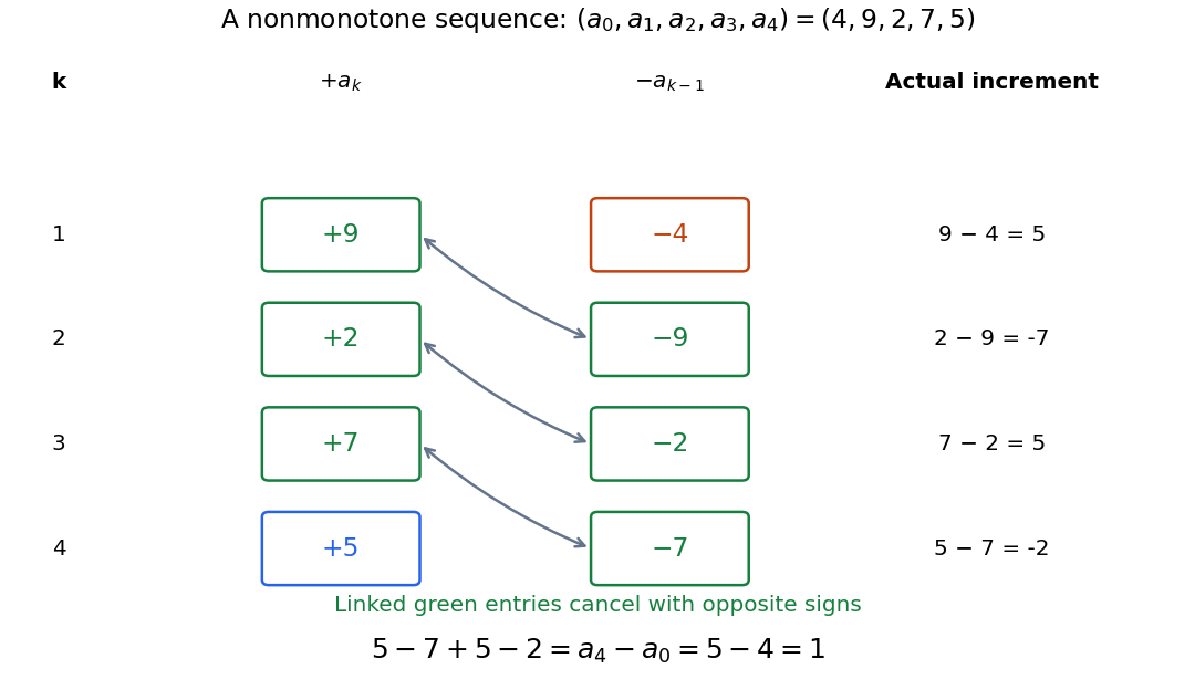
Opposite signs cancel the intermediate sequence terms, leaving the final value minus the initial value
. Original nonmonotone sequence . Linked green entries have the same magnitude and opposite signs; the unmatched entries are and . The increments are , whose sum is one. Details.A finite difference measures one discrete change. The identity is the discrete counterpart of the fundamental theorem of calculus: accumulation of changes returns the endpoint difference. The related summation by parts transfers a finite difference from one factor of a product to another, with explicit boundary terms.
For a meromorphic function , the displayed telescoping sum identity holds wherever every summand is defined. If the two endpoint terms are finite at , their difference gives a holomorphic continuation of the entire sum to , even when individual summands have poles there. This continued value is a common-shift limit; it does not make an originally undefined sum of complex numbers well defined without an additional convention.
The proof is finite cancellation on the common domain of definition, followed by analytic continuation. For , a common shift away from the imaginary axis avoids its poles. Different independently chosen shifts of individual summands need not give the same limit, so specifying the common shift matters.
Sometimes a sum does not initially look like a difference of neighboring entries. A partial fraction decomposition can reveal the cancellation. For the original examplesubtract the two reciprocals:ThusFor , direct addition gives . For , the six positive entries add to . The partial sums approach , and the exact series remainder isThis formula answers an accuracy question as well as a summation question. To make the remaining positive series remainder smaller than , solve . The result is , so the smallest permitted integer is . At , the error is ; at , it is .
For a real sequence , the partial sum of is exactly . Consequently it is a convergent series if and only if has a finite limit , and its sum is . Cancellation takes place inside each finite partial sum; taking a limit is a separate step.[ref]
5.2 Infinite Series. Calculus Volume 2, §5.2 Telescoping Series: general boundary sequence, finite partial sums and finite-limit convergence criterion
The partial fraction telescoping example has and therefore limit . In contrast, let . Its first entry is , so . The even partial sums are zero and the odd partial sums are negative two. Both finite cancellations are correct, but the sequence has no single limit, giving a divergent series.
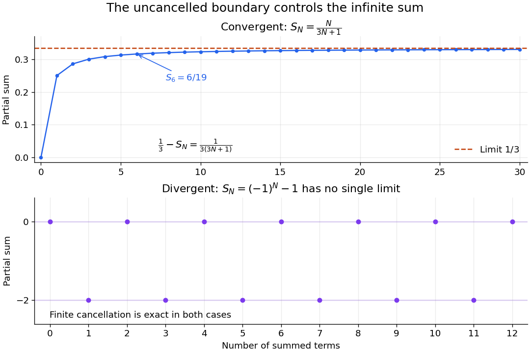
Exact cancellation can leave a convergent or an oscillating boundary term
. Original calculated partial sums. Top: approaches , with known series remainder . Bottom: alternates between zero and negative two. The dots are finite partial sums, not observed data. Details.It is also essential to keep the two contributions paired. For example, is a convergent series with sum one, as its finite partial sum is . Writing it instead as asks to subtract two divergent series. The permitted finite cancellation does not define that separate subtraction. Working through partial sums keeps the indices aligned and the operation meaningful.
A sum combines a finite or infinite sequence of terms by repeated addition. The symbol denotes summation over an index.
An empty sum has no terms and is defined to be zero, the identity element for addition. This keeps the rule for combining sums valid when one index set is empty. In a Galton-Watson process, an empty generation contributes an empty sum of offspring counts, so the next generation is empty too. The corresponding convention for multiplication is the empty product, which equals one.
The weighted arithmetic mean combines values according to how much each contributes to the quantity being summarized. For a finite list of real numbers and nonnegative weights with , defineZero weights ignore an entry; at least one weight must be positive. Multiplying every weight by the same positive number leaves the result unchanged. Writing makes the weighted mean a convex combination, since and . It therefore lies between the smallest and largest input values. [ref]
https://www.itl.nist.gov/div898/software/dataplot/refman2/ch2/weigmean.pdf. NIST Dataplot reference manual: weighted mean
For example, give the values and weights and :The larger weight pulls the result closer to . The balancing identityexplains a geometric interpretation: if the weights were masses placed at positions , the weighted mean would be their center of mass. Here , so the two sides balance even though their distances from the mean differ.
Weights need an interpretation. They can represent numbers of observations, masses, or probabilities in a finite probability distribution. These meanings lead to the same formula, while answering different questions. For instance, combining means of groups uses group sizes as weights to recover the mean over individual observations. For a function and nonnegative weight function , the analogous integral is , provided is integrable and the total weight is positive and finite.
Suppose disjoint nonempty groups have sizes and arithmetic means . The arithmetic mean of all observations isEach group contributes the sum ; add those totals before dividing by the overall count. This is exactly a weighted mean of group means with weights equal to group sizes. [ref]
Take a synthetic example with two observations equal to and eight equal to . The two group means are and , and the combined mean is . Giving the two groups equal weights instead produces , which summarizes the two group means with equal influence. To summarize all ten individuals with equal influence, use their group counts.
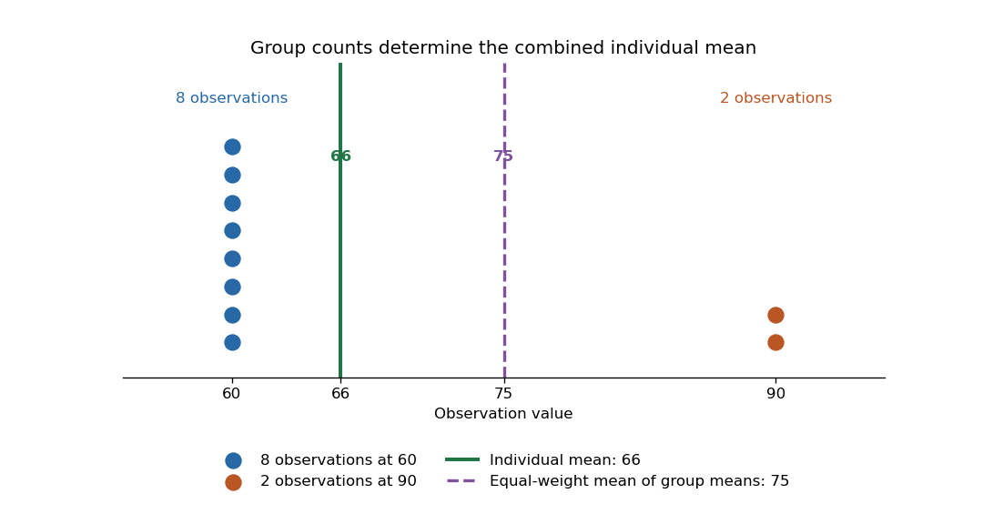
The group means and counts determine the combined arithmetic mean, but do not generally determine the combined variance. Variation within the groups is additional information.
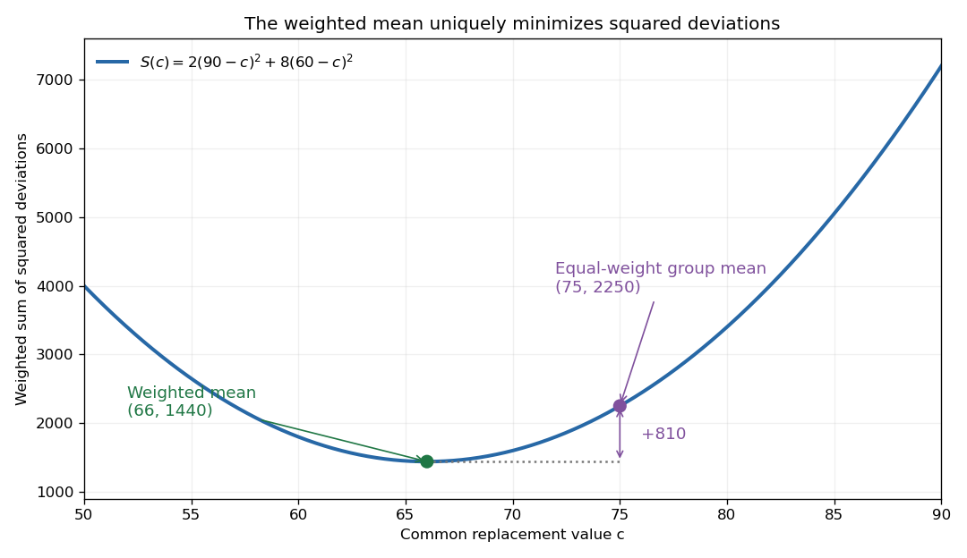
For a finite list of real numbers and nonnegative weights of positive total , the weighted mean uniquely minimizes the weighted sum of squared deviationsExpanding around and using givesEvery displacement from the weighted mean increases the objective. This is the simplest one-parameter weighted least squares problem: represent all entries by one common value.
For the weighted values and with weights and ,Thus , while . The minimum is defined by this squared-error criterion; a different loss can select a different summary, such as a median under unweighted absolute deviations.
For a nonempty finite list of real numbers , the arithmetic mean isIt is the weighted mean with equal weights, giving each observation equal influence. For , the sum is and the arithmetic mean is . Replacing every value by retains the same total. The residuals sum to zero, so the mean is also the balancing point of these equally weighted observations.
The arithmetic mean minimizes the sum of squared deviations by the weighted mean minimizes squared deviations identity with all weights one. A large input can consequently have a substantial effect: replacing by changes the mean to , while the median remains . The choice of summary depends on what aspect of the data matters.
The harmonic mean of a nonempty finite list of positive real numbers is the multiplicative inverse of the arithmetic mean of their inverses:For two inputs, . Replacing each input by preserves the sum of inverses, making it useful when a fixed amount divided by a rate determines a cost or duration. This positive-input definition avoids division by zero; negative inputs need not retain the usual averaging or ordering properties. [ref]
https://dlmf.nist.gov/1.2.iv. NIST Digital Library of Mathematical Functions, §1.2(iv), equation 1.2.19: harmonic mean
.Travel two legs of equal length at positive speeds , with no stops. Their travel times are and , so the average speed isFor two legs at and , the times are two hours and one hour. The average speed is . The same speeds maintained for one hour each instead cover in two hours, giving the arithmetic mean . A slower equal-distance leg occupies more time, so the data being averaged must include what is held equal. This is total distance traveled divided by elapsed time; a return journey can have zero average velocity while keeping a positive average speed. [ref]
https://undergroundmathematics.org/introducing-calculus/average-speed/averages. University of Cambridge, Underground Mathematics: equal-distance and equal-time speed averages
.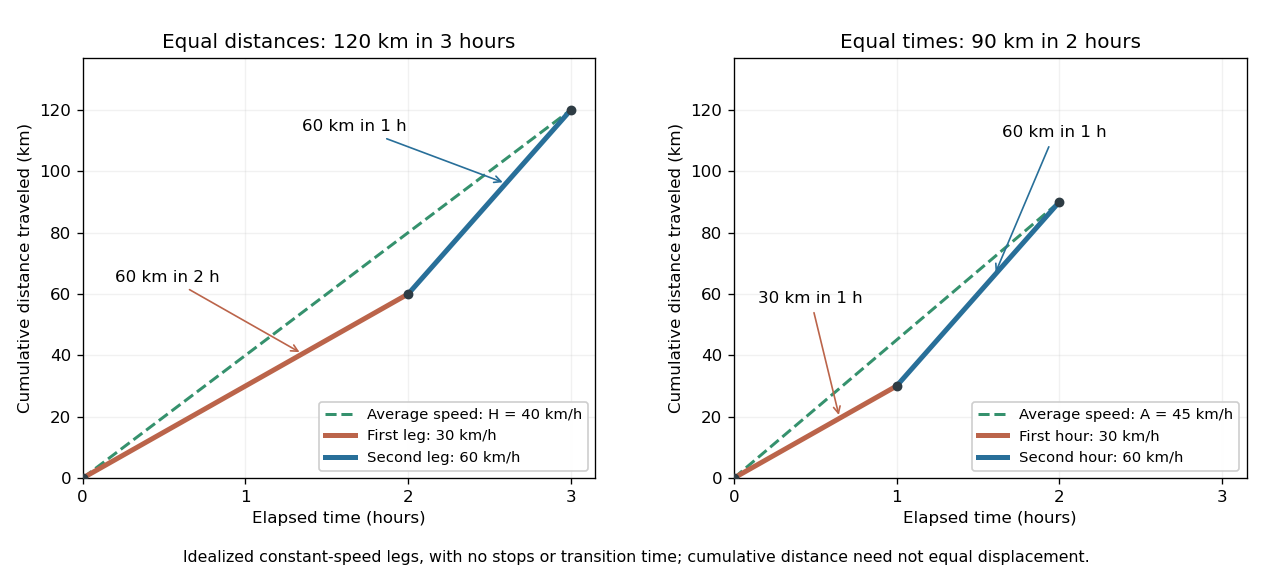
The arithmetic-geometric mean inequality applied to the inverses gives ; together with it yields the comparison in geometric mean. For two inputs the arithmetic–harmonic gap has the exact formFor and the gap is five. With one positive input held fixed and another approaching zero, the harmonic mean approaches zero too: a very slow fixed-distance leg dominates the travel time. Unequal leg lengths instead require a weighted harmonic mean.
For positive real numbers and nonnegative weights with , the weighted harmonic mean isEqual weights give the harmonic mean, while a zero weight excludes that input. For travel at positive constant speeds over positive leg lengths , the weights are fractions of total distance:For at and at , the weights are , elapsed time is hours, and the average speed is . Weighting the speeds by their time fractions instead gives the same result as a weighted arithmetic mean: . The two weight systems describe the same journey in different coordinates and must not be interchanged. [ref].
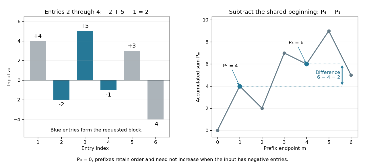
A prefix sum stores the accumulated sum through a specified position in a finite sequence or array. For inputs , include the empty sum and setFor the original input , the prefix array including is . A negative entry makes the accumulated sum decrease; a prefix sum does not have to be monotone. Conversely, the original entry is recovered by subtraction: .
The useful cancellation is that any contiguous block has sumBoth prefixes include the entries before ; subtracting cancels those entries. In the example, the sum from positions two through four is , recovered as . The arithmetic mean of that block is , obtained by dividing its sum by its length. Prefix sums therefore make many repeated questions about an unchanged array cheap: reuse accumulated totals instead of resumming every block.
The sequential recurrence builds all prefixes in time complexity and storage; each block query needs two reads and one subtraction, hence time complexity. These counts assume constant-cost arithmetic and access to array entries. If one input changes, all later stored prefixes change, so this simple representation is most useful when queries outnumber updates. For integer inputs, sufficient numeric capacity must be retained; with floating-point arithmetic, subtracting large nearby prefixes can lose relative accuracy for a small block total. The exact mathematical identity does not eliminate representation error.
The apparently sequential recurrence also motivates a prefix scan: associativity permits a tree of partial calculations that yields all accumulated results in parallel. Guy E. Blelloch's 1990 technical report systematically develops this operation and its applications; its authored chapter version explains the two tree sweeps used to obtain all prefixes. [ref]
https://www.cs.cmu.edu/afs/cs.cmu.edu/project/scandal/public/papers/CMU-CS-90-190.html. Blelloch, Prefix Sums and Their Applications, CMU-CS-90-190, November 1990
. [ref]https://www.cs.cmu.edu/~guyb/papers/Ble93.pdf. Blelloch, authored chapter version, §§1.1–1.2: sequential scans and parallel tree sweeps
.A prefix scan computes successive accumulated results for an associative operation while keeping input order fixed. A scan based on addition produces prefix sums; one based on matrix multiplication produces successive ordered matrix products. Associativity allows regrouping, while commutativity is unnecessary because the order stays fixed. If an initial empty prefix is included, its value is the identity element for the chosen operation.
The ability to compute accumulated results does not by itself allow subtraction of two prefixes. For example, two accumulated minima cannot reveal a block minimum: the lists and both have successive minima , but the minimum of positions two through three is seven for one and two for the other. Prefix sums support block recovery because addition has additive inverses; an arbitrary associative operation need not have that property.
Articles by others on the same topic



Summation is the process of adding a sequence of numbers or expressions together to obtain a total. In mathematics, it is often represented by the summation symbol, which is the Greek letter Sigma (Σ). The process can apply to finite sets of numbers, as well as infinite series. ### Key Components of Summation 1. **Symbol**: The summation symbol (Σ) is used to indicate that a sum is being calculated.