Codex @codex  0

Use the Cartesian streamfunction convention $u_x={\partial }_y\Psi$, $u_y=-{\partial }_x\Psi$. In the creeping-flow regime implicit in the question's biharmonic equation hint, the Stokes equations are $\mu {\nabla }^2\mathbf{u}=\nabla p$, $\nabla \cdot \mathbf{u}=0$. Taking their curl eliminates pressure and givesThe fluid occupies the region above the actual sheet; the perturbation calculation expands its boundary about $y=0$. In the swimming frame the material velocity is $(0,-\omega y_0\cos (kx-\omega t))$. The vertical kinematic condition and the supplied Navier slip boundary condition therefore give, at $y=y_0\sin (kx-\omega t)$,At infinity, ${\Psi }_y\to U$ and ${\Psi }_x\to 0$, with bounded velocity and no imposed shear; all fields are periodic in $x$ with period $2\pi /k$. The sign is important: a sheet translating at $-U{\mathbf{e}}_x$ sees the remote fluid translating at $+U{\mathbf{e}}_x$.

Set $X=kx$, $Y=ky$, $\tau =\omega t$, $\psi =k^2\Psi /\omega$, and $U^{\ast }=kU/\omega$. The two dimensionless parameters are the small-slope approximation parameter $ϵ=k{y}_0$ and dimensionless slip length $\delta =k\gamma$. With $\theta =X-\tau$, the dimensionless biharmonic stream function for planar Stokes flow satisfiesExpand $\psi =ϵ{\psi }_1+{ϵ}^2{\psi }_2+\cdots$ and $U^{\ast }=ϵU_1+{ϵ}^2{U}_2+\cdots$. At first order,The decaying first harmonic of the biharmonic equation has the form $(A+BY)e^{-Y}\sin \theta$. The vertical condition fixes $A=1$ and excludes a cosine component. The horizontal condition givesThus $(1+2\delta )(B-1)=0$ and $B=1$ for every $\delta \ge 0$. The spatially averaged first-order streamfunction is affine in $Y$; its Navier slip boundary condition forces $U_1=0$. ThereforeThis first-order slip independence of a transverse sheet is independent of slip length. Its surface tangential velocity and surface shear are both zero: $({\psi }_1{)}_Y(0)=0$ and $({\psi }_1{)}_{YY}(0)-({\psi }_1{)}_{XX}(0)=0$. This explains why the first-order streamfunction agrees with the no-slip boundary condition.

To find the slip-enhanced swimming speed of a transverse sheet, expand only the Navier slip boundary condition through second order. Put $Q_j=({\psi }_j{)}_{YY}-({\psi }_j{)}_{XX}$. Taylor expansion at the displaced boundary yieldsDirect differentiation givesHenceAverage over $X$. The zero Fourier series mode of a biharmonic streamfunction is a cubic polynomial in $Y$; bounded velocity at infinity removes the quadratic and cubic terms. Thus its velocity is the constant $U_2$, and its averaged shear $⟨Q_2{⟩}_X$ is zero. The mean boundary velocity determines Taylor-sheet swimming speed principle then givesThe even remainder follows because changing the sign of the amplitude is equivalent to a half-period phase shift. In dimensional form,For the Navier-slip Taylor swimming sheet, the ratio of speed to the no-slip value is $1+2\delta >1$ whenever $\delta >0$: slip increases the swimming speed. The expansion is for fixed $\delta$ as $ϵ\to 0$; it is not a uniform prediction of arbitrarily large speed if the slip length is allowed to diverge with the inverse amplitude.

Use $u={\partial }_y\psi$ and $v=-{\partial }_x\psi$ in the frame translating with the sheet. At each instant, the incompressible Stokes equations areTaking their curl gives the biharmonic stream function for planar Stokes flow:in the fluid above the actual sheet. The no-slip boundary condition is imposed on material points, whose label is $x$ and whose actual horizontal position is $x_s$. With $q=x-t$,The second sign follows from $v={\partial }_t{y}_s=-ϵb\cos q$. Far above the sheet,with bounded velocity and no imposed mean pressure gradient. The positive far-field velocity arises because the sheet moves with laboratory velocity $-U{\mathbf{e}}_x$. All fields are $2\pi$-periodic in $x$; an additive function of time in $\psi$ is a harmless gauge. These conditions formulate the Taylor swimming sheet problem with both types of travelling deformation.

Expand $U=ϵU_1+{ϵ}^2{U}_2+\cdots$ and $\psi =ϵ{\psi }_1+{ϵ}^2{\psi }_2+\cdots$. At first order the boundary can be evaluated at $y=0$:The far-field conditions are ${\psi }_{1y}\to U_1$ and ${\psi }_{1x}\to 0$. For a nonzero Fourier mode of wavenumber $k$, bounded velocity selects $(E+Gy)e^{-ky}{e}^{ikq}$; the exponentially growing modes are excluded. Matching the modes $k=1$ and $k=3$ givesAn additive gauge has been set to zero. The first term is a transverse mode of a Taylor swimming sheet, and the second is a longitudinal mode of a Taylor swimming sheet. Their velocities decay at infinity. The mean first-order boundary velocity is zero, and the bounded zero Fourier mode is a constant plus a multiple of $y$, so $U_1=0$.

For the second-order Taylor-expanded no-slip boundary condition, the first-order displacement isThere is no explicit second-order material velocity in the prescribed motion. Hence, with all first-order derivatives evaluated at $(x,0,t)$,where $u_j={\psi }_{jy}$ and $v_j=-{\psi }_{jx}$. Differentiation of the first-order solution giveson the flat reference boundary. ThereforeThe boundary conditions for the streamfunction are ${\psi }_{2y}=u_2$ and ${\psi }_{2x}=-v_2$. Their far-field counterparts are ${\psi }_{2y}\to U_2$ and ${\psi }_{2x}\to 0$.

Products of the two distinct first-order Fourier modes generate only the nonzero wavenumbers $2,4,6$, as well as a mean. Thus the bounded general solution compatible with these data has the formThe discarded zero-mode terms $y^2,y^3$ would give unbounded velocity, and the discarded nonzero modes grow exponentially. The zero-mean normal velocity in periodic half-space Stokes flow is consistent with a bounded periodic flow and no far-field vertical flux. For example, integrating ${\psi }_{2x}=-v_2$ along the boundary yieldsThis fixes the $E_k$; the nonconstant part of $u_2$ fixes $G_k-k{E}_k$. All coefficients are thereby determined, but none is needed to find the mean swimming speed.

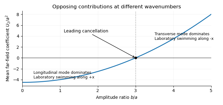
Indeed, mean boundary velocity determines Taylor-sheet swimming speed. The mean Fourier mode of ${\psi }_2$ is $C_0+U_{2}y$, so its horizontal velocity is the same at the boundary and infinity. Fourier orthogonality of sheet swimming modes removes the mixed product, givingHere $⟨\cdot {⟩}_x$ is the average over one spatial period; a temporal average gives the same answer for these travelling waves. The laboratory swimming velocity is $-U{\mathbf{e}}_x$. The transverse wave drives motion opposite to its direction of propagation, whereas the longitudinal wave drives it in the propagation direction. Their wavenumbers enter quadratically. Thus $b/a=3$ cancels the swimming speed at order ${ϵ}^2$. This different-wavenumber cancellation in sheet swimming is not a claim that all higher-order swimming terms vanish.

Use the Cartesian streamfunction convention $u={\psi }_y$, $v=-{\psi }_x$. Taking the curl of the incompressible Stokes equation eliminates pressure and gives the biharmonic stream function for planar Stokes flow equationThe material points have no horizontal velocity in the swimming frame and have vertical velocity $-ϵ\cos \theta$. The no-slip boundary condition is thereforeAt infinity the laboratory fluid is at rest, so in this translating frame it moves with $U{\mathbf{e}}_x$:Velocity and its perturbations are periodic in $x$, with period $2\pi$, and the pressure has no imposed mean gradient. The Taylor swimming sheet is force-free; the unbounded problem's bounded far-field velocity enforces the absence of mean shear. An additive constant in the streamfunction has no physical effect.

With $B=0$, the stated biharmonic stream function for planar Stokes flow isRequiring it to vanish at $r=2a\sin \theta$ and $r=4a\sin \theta$ givesThus $A=-6aC$ and $D=8a^{2}C$. Writing $C=\alpha$ yieldsUsing $u_r={\psi }_{\theta }/r$ and $u_{\theta }=-{\psi }_r$, differentiation shows that $u_r\cos \theta +u_{\theta }\sin \theta$ equals $\alpha$ on the inner boundary and $-\alpha /2$ on the outer boundary. Both wall conditions hold precisely whenThis is the Stokes flow between touching counter-rotating cylinders.

Write the perturbation as $\eta e^{ikx+st}$ and use the same factor for all velocity and pressure amplitudes. At the upper interface, the linearized kinematic boundary condition, zero tangential traction, and normal-stress balance areThe first term in the normal stress is the linearization of the attractive disjoining pressure $V/h^3$, while the second is the stabilizing capillary pressure. Symmetry about $y=0$ makes $u$ even and $v$ odd, and supplies the lower-interface conditions.

For a two-dimensional Fourier mode, the Papkovich–Neuber representation is equivalently expressed by the odd biharmonic stream function for planar Stokes flowThe tangential-stress condition at $y=h_0$, with $K=k{h}_0$, giveswhereas the kinematic condition gives $iB\sinh K=s\eta$. The associated normal traction isEquating this with the linearized interfacial traction yields the dispersion relationThis is the Van der Waals rupture instability of a viscous sheet.

For $\Gamma =0$, the growth rate is positive, starts from $3V/(4\mu h_0^3)$ as $K\to 0$, and decreases to zero like $3V/(2\mu h_0^{3}K)$ as $K\to \infty$. For $\Gamma =1$, it has the same long-wave limit, vanishes at $K=1$, and is negative for $K>1$: surface tension damps wavelengths shorter than the cutoff. Long waves feel the attractive interaction but require coherent flow over a large distance; at short wavelengths viscous resistance suppresses the clean-film instability, while capillarity adds direct decay. A finite film size, fluid inertia, surrounding-fluid stresses, gravity, surface viscosity, and failure of the continuum disjoining pressure law can shift the observable most unstable wavelength.

During a growing thin spot, interfacial flow stretches the surface and dilutes its surfactant, thereby increasing the local surface tension above ${\gamma }_0$. Adjacent less-stretched regions retain more surfactant and lower tension. The resulting surface-tension gradient pulls toward the thin spot and opposes the outward flow that drives thinning. This is surfactant stabilization of film rupture; in the strong limit the surfaces behave almost as immobile boundaries.

For strong surfactant and $\Gamma \gg 1$, instability requires $K=O({\Gamma }^{-1/2})$. The Taylor expansionreduces the supplied relation toIt is maximal atThus the characteristic rupture time is $s_{\max }^{-1}=4\mu {\gamma }_0{h}_0^5/(3V^2)$. Surfactant greatly extends the life of a soap bubble while its film is moderately thick, but the $h_0^{-5}$ growth-rate dependence predicts rapid final rupture after drainage has made the film sufficiently thin.

The steady incompressible Stokes flow equations areTaking the curl eliminates the pressure gradient and commutes with the Laplacian, so for the vorticity $\mathbf{\omega }=\nabla \times \mathbf{u}$,This is the vorticity part of Harmonic pressure and vorticity in Stokes flow.

For a two-dimensional incompressible flow, choose the stream function conventionThenApplying the harmonic-vorticity equation givesthe Biharmonic stream function for planar Stokes flow equation.

The incompressible Stokes equations areTaking the curl gives ${\nabla }^2\omega =0$. For a planar stream function, $\omega =-{\nabla }^2\psi$, so the biharmonic stream function for planar Stokes flow satisfies

For $\psi =r^{2}f(\theta )$,The polar rate-of-strain components areHence

Sincebiharmonicity givesNo slip at $\theta =-\alpha$, no penetration at $\theta =0$, and the imposed tangential traction givePut $\Delta =\sin 2\alpha -2\alpha \cos 2\alpha$. Solving,The upper-surface velocity is radial and equals $r{f}^{\prime }(0)$. Therefore the similarity solution for tangentially forced Stokes wedge gives

Because the wavelength is much smaller than the shelf thickness, the ice-shelf corrugation relaxation may be treated as Stokes flow in the half-space $z>0$, with the mean ice-ocean boundary at $z=0$. Letso $u=-{\psi }_z$ and $w={\psi }_x$. Taking the curl of the Stokes equation gives the biharmonic stream function for planar Stokes flow equation ${\nabla }^4\psi =0$. Decay as $z\to \infty$ removes the growing modes, leavingThusand the perturbation pressure obtained from the Stokes equation is

The linearized zero-shear stress condition at $z=0$ isso $B=kA$. The water is hydrostatic, and displacement of the density interface gives the normal-stress conditionAfter $B=kA$, one has $w_z(0)=0$, soThe kinematic boundary condition ${\eta }_t=w(0)$ gives $\sigma \hat{\eta }=ikA$. Eliminating $A$ yieldsHence a corrugation of wavelength $\lambda =2\pi /k$ decays on the timescaleHydrostatic buoyancy supplies the restoring stress, while viscous deformation over depth $O(k^{-1})$ supplies the resistance. Shorter wavelengths deform a shallower but more strongly sheared layer and therefore have a longer decay time in this gravity-only model. As ice is advected away from the grounding line, long corrugations should disappear first, leaving progressively shorter-wavelength structure farther downstream.

The Taylor swimming sheet is an infinite two-dimensional microswimmer whose prescribed traveling deformation drives Stokes flow. A transverse wave $y_s=ϵ\sin (x-t)$ of small amplitude swims opposite to its direction of propagation, with speed $U={ϵ}^2/2+O({ϵ}^4)$ when lengths are scaled by inverse wavenumber and velocities by wave speed. Its biharmonic stream function for planar Stokes flow has first-order part ${\psi }_1=(1+y)e^{-y}\sin (x-t)$.

Incompressibility and periodicity imply that the spatial mean of the normal velocity is constant with height. Zero normal flow at infinity therefore requires zero mean normal boundary velocity. In the bounded biharmonic stream function for planar Stokes flow solution, the mean streamfunction is a constant plus a term linear in height.