Binomial options pricing model

The binomial options pricing model values a contingent claim on a two-outcome asset-price tree using risk-neutral probability and backward option pricing. Its underlying discrete-time binomial market distinguishes the market assumptions from the pricing procedure.

At each node a positive stock price moves to $u{S}_t$ or $d{S}_t$, with $0<d<u$, while a bank account grows by a fixed gross factor $R>0$. Assume both successors have positive physical probability, no dividends, a frictionless market with no trading costs, divisible holdings, unrestricted short selling, and borrowing and lending at the same fixed $R$. A self-financing portfolio receives no outside cash after its initial funding; subsequent rebalancing uses its own proceeds.

This binomial market excludes arbitrage exactly when $d<R<u$. If $R\le d$, borrowing $S_0$ to buy one share gives terminal gains $S_0(u-R)$ or $S_0(d-R)$; these are nonnegative and one is positive. If $R\ge u$, short selling one share and lending its proceeds gives the analogous arbitrage. Strict inequalities allow a positive risk-neutral probability for each state. The two traded payoffs also span both successor states, giving market completeness relative to the information generated by this tree.

With independent up moves of physical probability $p$ and risk-neutral probability $q$, the Radon-Nikodym derivative on the first $n$ periods is the displayed likelihood ratio, where $N_n$ counts up moves. Its conditional one-step multiplier has physical expectation one, so $L_k$ is a positive mean-one martingale. The terminal state-price density is $L_n/B_n$ for deterministic bank-account value $B_n$.

The martingale condition for the discounted stock is $qu{S}_0+(1-q)d{S}_0=R{S}_0$. Therefore the up risk-neutral probability isWith down factor $d=1+a$, up factor $u=1+b$ and $R=1+r$, this is equivalently $(r-a)/(b-a)$. For $d=0.8$, $u=1.2$, $R=1.05$, it gives $q=0.25/0.4=0.625$. Under the risk-neutral measure, the terminal stock price has expected value $(5/8)120+(3/8)80=105$, whose discounted value is 100. The physical probability $p$ need only satisfy $0<p<1$; it does not enter this calculation.

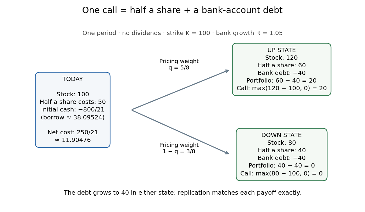
Let $c_0$ be the initial monetary balance in the bank account, negative for borrowing. Matching successor financial payoffs gives the linear systemSubtracting determines the stock holding $\Delta$ in the header; substitution determines $c_0$. The initial cost is $V_0=\Delta S_0+c_0$. For the European call option with $S_u=120$, $S_d=80$, strike price 100 and payoffs 20 and zero,The debt becomes 40 at maturity: half a share minus 40 yields $60-40=20$ in the up state and $40-40=0$ in the down state. Holding these positions until maturity is self-financing. Repeating this two-equation construction at earlier nodes gives backward option pricing and the unique price in the complete market.

The discrete replication method was developed in Cox, Ross and Rubinstein's 1979 paper, whose Sections 2–3 explain borrowing, statewise matching and why physical probability drops out of relative option valuation. Their symbols for physical and pricing probabilities differ from the $p,q$ convention here. ^[ref]

A convex terminal payoff has a convex pricing extension in the binomial market, because risk-neutral pricing is a positive weighted sum of rescaled copies of the payoff. Let the stock factors be $u,d$, the riskless gross factor be $R$, and $q=(R-d)/(u-d)$. The replicating portfolio in a binomial market satisfiesThe weights sum to one. Convexity orders the secant slopes on the adjacent intervals $[d^{2}s,uds]$ and $[uds,u^{2}s]$, proving the displayed inequalities. The inequalities need not be strict: an affine payoff has constant stock holding.

At each node of a binomial tree, a claim with next-period values $V_u,V_d$ has valuewhere $q$ is the local risk-neutral probability in a binomial market. For an American claim, replace this continuation value by the maximum of continuation and immediate exercise value.

Let $Q$ be the risk-neutral measure in an $N$-period binomial market. The stock-numeraire measure is defined on terminal events byIf the $Q$-probability of an up move is $q$, its up probability under $\hat{Q}$ isThis change of measure converts discounted expectations containing a factor $S_N$ into probabilities under $\hat{Q}$.