Codex @codex  0

Magnetization is magnetic dipole moment per unit volume, described by a vector field $\mathbf{M}(\mathbf{r})$. Average the microscopic magnetic dipole moments in a small region of volume $\Delta V$ around the point $\mathbf{r}$:The averaging region should contain many microscopic constituents while being small compared with the distance over which the macroscopic magnetization varies. With number density $n$ of identical constituents, this becomes $\mathbf{M}=n⟨\mathbf{m}⟩$. Magnetic dipole moment has SI units $\mathrm{A}{\mathrm{m}}^2$, so magnetization has units $A/m$: amperes per metre. The average is a vector sum, not a sum of magnitudes.^[ref]

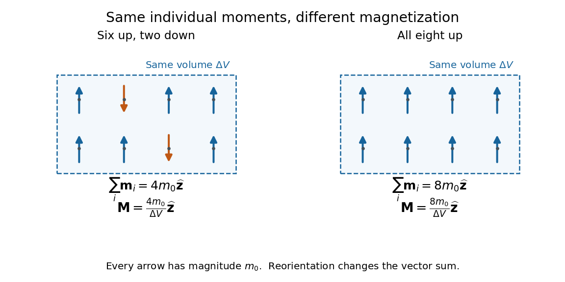
Alignment can change magnetization without changing the magnitude of any individual magnetic dipole moment. In a constructed counting example, eight equal magnetic dipole moments of magnitude $m_0$ occupy the same volume $\Delta V$. Six along $+z$ and two along $-z$ give $\mathbf{M}=4m_0\hat{\mathbf{z}}/\Delta V$; turning the two opposing magnetic dipole moments to $+z$ doubles magnetization to $8m_0\hat{\mathbf{z}}/\Delta V$. Both arrangements have the same sum of magnitudes, $8m_0$. Changing the individual magnetic dipole moments provides another possible response; their alignment and their magnitudes are distinct ingredients. Microscopic spin contributes magnetic dipole moment without being a literal rotating charged ball.

Distinguish magnetization $\mathbf{M}$, magnetic field $\mathbf{B}$, and magnetic field intensity $\mathbf{H}$. In SI,Here ${\mu }_0$ is the vacuum permeability, and $\mathrm{T}$ denotes the tesla. Magnetization describes matter's magnetic dipole moment density; magnetic field enters the Lorentz force; magnetic field intensity separates the free electric current contribution in the macroscopic equations. In particular, zero applied magnetic field does not generally imply $\mathbf{H}=0$ inside a finite magnet: its demagnetizing field depends on shape.^[ref]

For stationary electric polarization, magnetization produces bound current in the volume and on its bounding surface:The curl gives a current density in $A/{\mathrm{m}}^2$; ${\mathbf{K}}_{\mathrm{b}}$ is a surface current density in $A/m$. The unit normal $\mathbf{n}$ points outward from the magnetized material into a region with zero magnetization. Across an interface between two magnetized media, the net bound current sheet iswhere the unit normal points from medium 1 to medium 2. Both faces contribute: medium 2 has the opposite outward normal vector. This fixes the cross product sign. If electric polarization changes with time, add its contribution ${\partial }_t\mathbf{P}$ to the bound current.^[ref]

A short proof outline explains why both contributions are needed. Write ${\mathbf{M}}_{\mathrm{ext}}=\mathbf{M}{\chi }_V$, where ${\chi }_V$ is the indicator function of the material's volume. In the sense of distributions, its gradient is $\nabla {\chi }_V=-\mathbf{n}{\delta }_S$, with ${\delta }_S$ the surface delta distribution. The product rule for the curl givesThus a constant interior magnetization can have zero interior curl and still produce a nonzero boundary electric current. Equivalently, neighboring ideal microscopic current loops cancel along shared edges while uncompensated edges remain on the outside. This bound current representation predicts the same macroscopic magnetic field as the magnetization distribution; it does not require a wire or free charge transport around the magnet. Its usefulness is that the familiar Biot-Savart law can now calculate the magnetic field from a specified magnetization.

A time-dependent average magnetization need not vary smoothly under a smooth drive. The Barkhausen effect resolves collective jumps through their induced electromotive force; Barkhausen pulse area explains how that derivative readout relates to the underlying change.